flowchart LR
    A[Raw FASTQ] --> B[QC + Adapter<br/>fastp/MultiQC]
    B --> C[Alignment<br/>bwa-mem2]
    C --> D[Add Read Groups]
    D --> E[Mark Duplicates<br/>GATK]
    E --> F[BQSR]
    F --> G[Contamination<br/>Check]
    G --> H[Mutect2]
    H --> I[Filter<br/>Calls]
    I --> J[Annotation<br/>VEP]

    %% Define the yellow style class
    classDef covered fill:#ffeb3b,stroke:#333,stroke-width:2px;

    %% Apply the class to specific nodes
    class B,H,I,J covered;
Cancer Variant Analysis
Introduction to Cancer Genomics and Variant Detection
2025-12-12
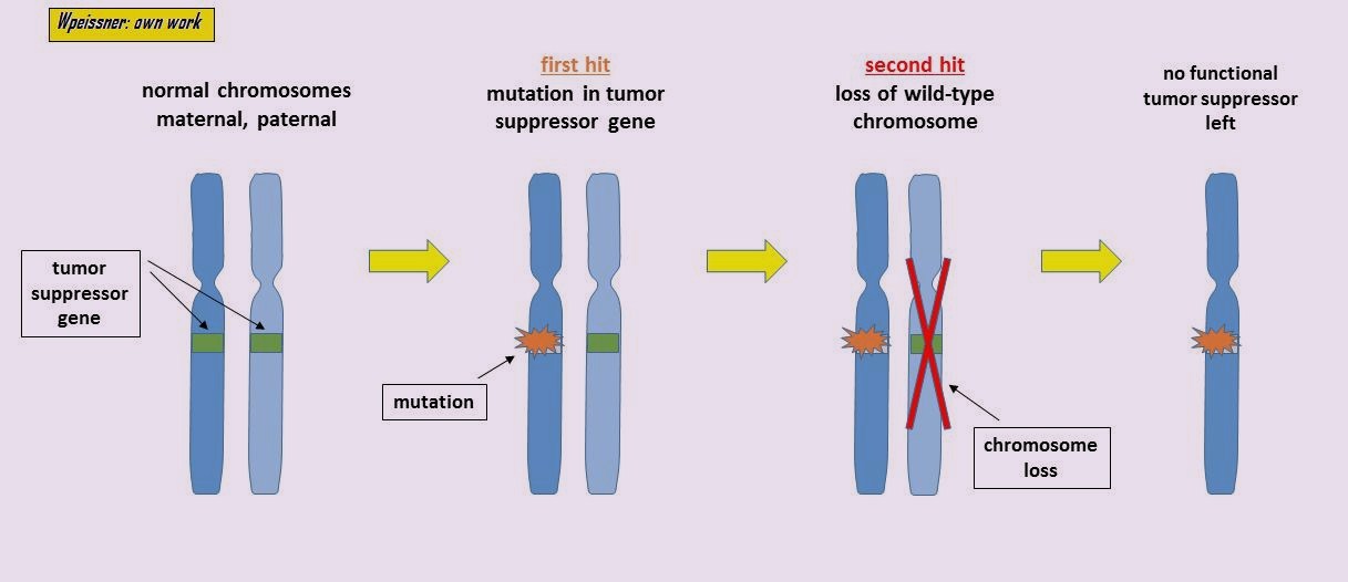
Cancer: A Disease of the Genome
Key characteristics:
- Abnormal cell growth - uncontrolled proliferation
- Invasive potential - ability to spread (metastasis)
- Initiated by acquired genomic mutations affecting cell growth regulators
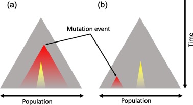
- Mutations occur stochastically, but rate influenced by environment
- Clonal evolution - natural selection of malignant cells
Driver vs Passenger Mutations
Cancer genomes typically harbor 2-8 driver mutations (Vogelstein et al., 2013), though this varies by cancer type. Pediatric cancers often have fewer drivers, while hypermutated adult cancers may have more. Drivers represent a small minority of total mutations.
Hereditary vs Sporadic Cancer
Sporadic (~90-95%)
- Acquired somatic mutations
- Accumulate during lifetime
- Environmental factors contribute
Hereditary (~5-10%)
- Inherited predisposition alleles
- BRCA1/2 (breast, ovarian)
- Lynch syndrome genes (colorectal)
- Still require somatic “second hits”
Clinical Relevance
Hereditary cancer syndromes have implications for family screening, risk reduction, and treatment options (e.g., PARP inhibitors for BRCA carriers).
Variant Terminology: Essential Definitions
Mutation: The process of change in DNA
Variant: A difference in DNA sequence compared to a reference (the outcome)
Somatic variant: Occurs only in specific cells/tissues - Not inherited - Arises during lifetime
Germline variant: Present in all cells - Can be passed to offspring - Present from conception
Polymorphism: Traditionally defined as variant >1% frequency in population (though “variant” is now preferred terminology)
Mutation vs Variant: A Practical Example
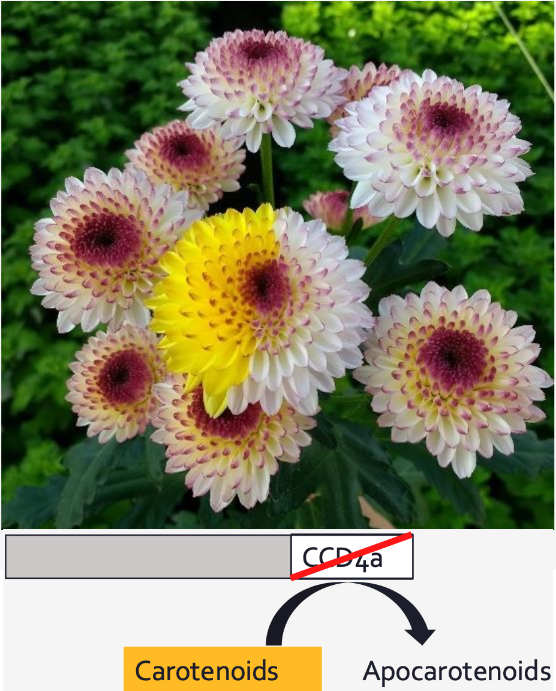
The Yellow Flower Example:
- Mutation: The change in DNA that caused petals to turn yellow
- Variant: The resulting DNA difference between yellow and white flowers
This is a somatic mutation - occurring during the plant’s development in one branch, analogous to somatic mutations in cancer.
The CCD4a gene mutation prevents breakdown of carotenoids, leading to yellow pigmentation.
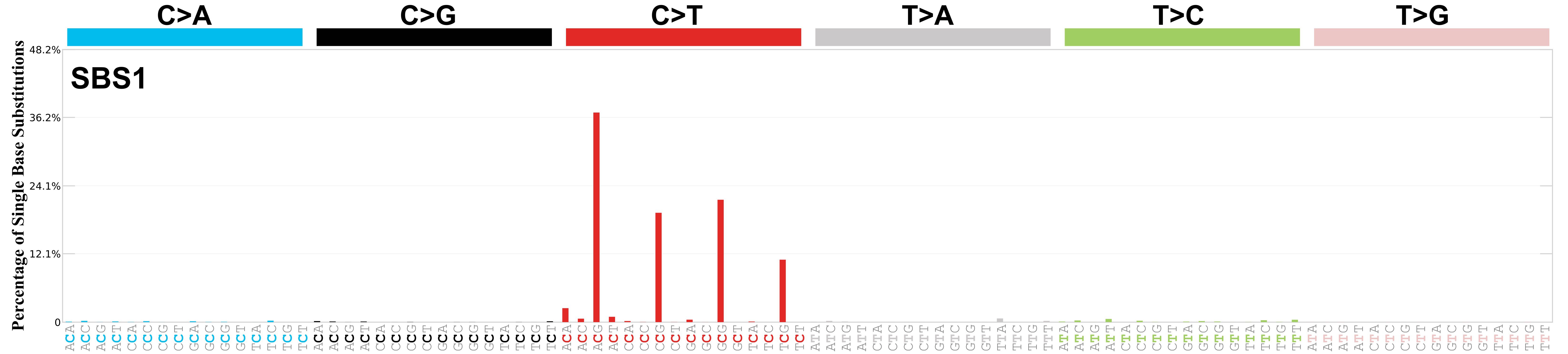
Mutational Signatures: Fingerprints of Mutagenesis
Each mutational process leaves a characteristic pattern:
Signature 1: Aging, C>T at CpG sites, Transition (Py \(\leftrightarrow\) Py)
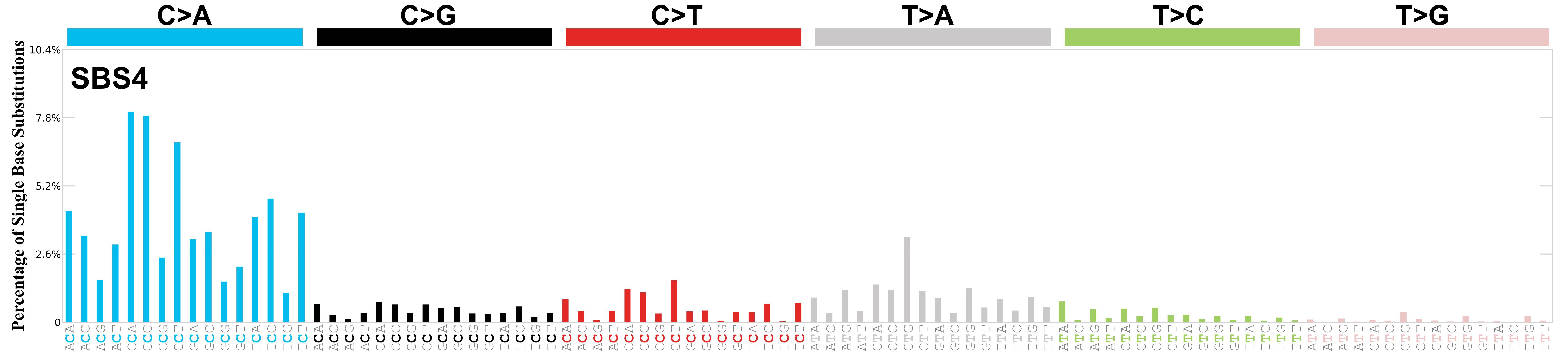
Signature 4: Tobacco smoking, C>A, Transversion (Py \(\leftrightarrow\) Pu)
Signature 6: Mismatch repair (MMR) deficiency
Signature 7: UV light, C>T at dipyrimidines, Transition
Clinical applications:
- Understanding tumor etiology (e.g. Signature 4, 7)
- Treatment selection (e.g., PARP inhibitors for HRD) (Signature 3)
- Immunotherapy response prediction (Signature 6)
Reference
Alexandrov et al. (2020) “The repertoire of mutational signatures in human cancer” - Nature
Sequencing Strategies for Cancer Genomics
Coverage strategies
- Whole Genome Sequencing (WGS)
- Complete genome coverage
- Detects all variant types
- Best for structural variants
- Whole Exome Sequencing (WES) (Bait Capture)
- Protein-coding regions only
- Cost-effective (
WES 100x: 25 M 2 x 100 bp
WGS 30x: 450 M 2 x 100 bp
) - Misses non-coding regions
- Custom panels (Bait Capture, mostly)
- Targeted cancer genes
- Deep coverage
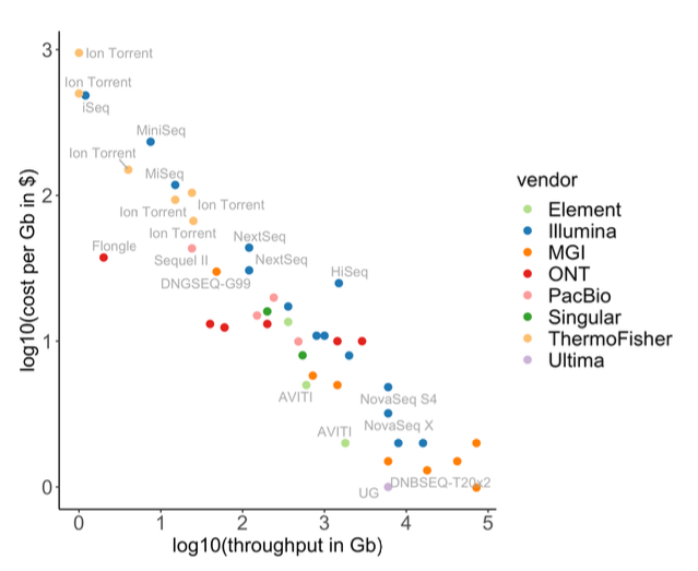
Sequencing technologies
Short reads (2x150bp standard):
- Illumina, MGI, Element, Ultima
- High accuracy, mature pipelines
Long reads:
- PacBio HiFi: >Q30 accuracy
- Oxford Nanopore: Q20+ with R10.4.1
- Superior for SVs and phasing
Depth Recommendations
WGS: 60-100x tumor, 30-40x normal WES: 100-200x ctDNA: 10,000-30,000x
Experimental Design: Tumor-Normal Pairs
The challenge: Tumor tissue is heterogeneous - contains: - Tumor cells - Immune infiltrates - Stromal cells - Normal tissue
Solution: Paired samples
- Tumor sample - from the malignancy
- Normal sample - typically blood
For hematological malignancies, use skin biopsy or buccal swab (blood IS the tumor!)
Tumor Purity
Typical tumor purity ranges from 30-80%. Samples below 20-30% purity may have insufficient power for reliable somatic variant detection. Consider pathologist review or microdissection.
Marking PCR Duplicates
Why it matters:
- Variant callers assume each read is an independent observation
- PCR/optical duplicates violate this assumption
- Can lead to false positive variant calls
Solution:
- Mark duplicates based on alignment coordinates
- Use Unique Molecular Identifiers (UMIs) for accurate deduplication - especially important for low-input and ctDNA samples
Tool: gatk MarkDuplicates

Somatic Variant Calling Challenges
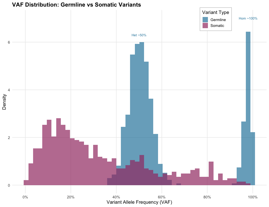
Germline calling assumes:
- Heterozygous: ~50% VAF (typically 30-70% due to technical variation)
- Homozygous: ~100% VAF
These assumptions fail in tumors:
- Variable tumor purity (30-80%, which is effectively contamination by normal cells)
- Clonal heterogeneity (subclones)
- Copy number alterations
- VAF can be anywhere from <1% to 100%
Additional challenges:
- Sequencing errors, alignment artifacts
- FFPE artifacts
- C>T/G>A deamination
- 8-oxoG which causes the G>T transversions
- Sample contamination
Let’s make an example (assuming diploid genome and CN=2)
1. The Ideal Case
Sample is 100% Tumor
If a mutation is heterozygous (1 of 2 alleles): \[\text{VAF} = \frac{1}{2} = \mathbf{50\%}\]
To a caller, this looks like a clear, standard germline variant.
2. Closer to reality
Sample is 40% Tumor (60% Normal)
The normal cells (wild type) dilute the signal. \[\text{VAF} = \frac{\text{Purity}}{2}\] \[\text{VAF} = \frac{0.40}{2} = \mathbf{20\%}\]
Real-world complications
Aneuploidy complicates this further: In real cases, copy number alterations can dramatically change expected VAF. For example, if the mutation is on a region with CN=4, the math becomes more complex.
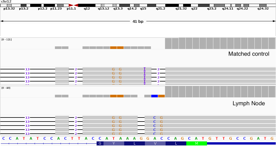
Tumor-infiltrated controls: Matched control samples can also be tumor-infiltrated, making it sometimes impossible to distinguish true somatic variants from germline or contamination.
Tumor Purity, Ploidy, and Clonality
Key concepts:
Tumor purity: Fraction of tumor cells in sample
Ploidy: Average copy number across genome (often >2 in cancer)
Clonal variants: Present in all tumor cells
Subclonal variants: Present in a subset of tumor cells
VAF interpretation examples:
- Pure tumor (100%), clonal het variant → VAF ≈ 50%
- 50% purity, clonal het variant → VAF ≈ 25%
- 50% purity, subclonal variant (20% of cells) → VAF ≈ 5%
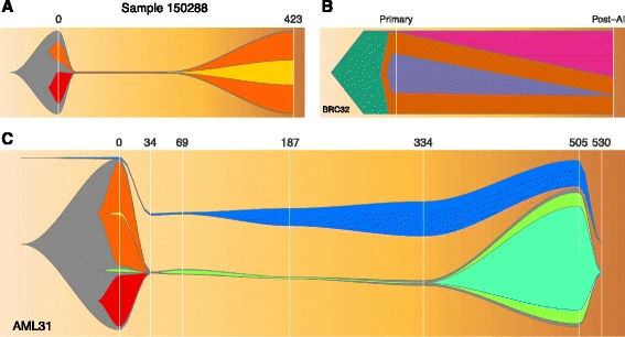
Clinical Relevance
Subclonal variants can become dominant after treatment selection pressure, leading to resistance.
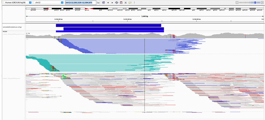
Structural Variation Detection
Types:
- Large insertions/deletions
- Translocations
- Inversions
- Complex rearrangements
Detection methods:
- Discordant read pairs
- Split reads
- Read depth changes
- Assembly-based approaches
Tools: Manta, Tiddit, GRIDSS2, DELLY, Sniffles2 (long reads)
Long Reads Advantage
Long-read sequencing (PacBio HiFi, ONT) dramatically improves structural variant detection, especially for complex rearrangements and insertions.
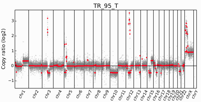
Copy Number Variation (CNV)
Characteristics:
- Gains or losses of genomic segments
- Full chromosome or arm-level events common
- Can cause Loss of Heterozygosity (LOH)
Detection approach:
- Calculate coverage in bins
- Normalize for GC content and mappability
- Compare tumor vs normal ratio
- Segment and call CNV regions
Tools: CNVkit, ASCAT, Control-FREEC, PURPLE
Clinical Example
ERBB2 (HER2) amplification in breast cancer determines eligibility for trastuzumab. MYC amplification is prognostic in many cancers.
Gene Fusions in Cancer
Mechanism:
- Chromosomal translocation
- Fusion of gene elements
- Creates chimeric transcripts
Detection data types:
- WGS (genomic breakpoints)
- WES (if breakpoints in exons)
- RNA-seq (fusion transcripts)
Detection method: Discordant alignments where paired reads map to different genes/chromosomes
Tools: Manta (DNA), STAR-Fusion, Arriba (RNA-seq)
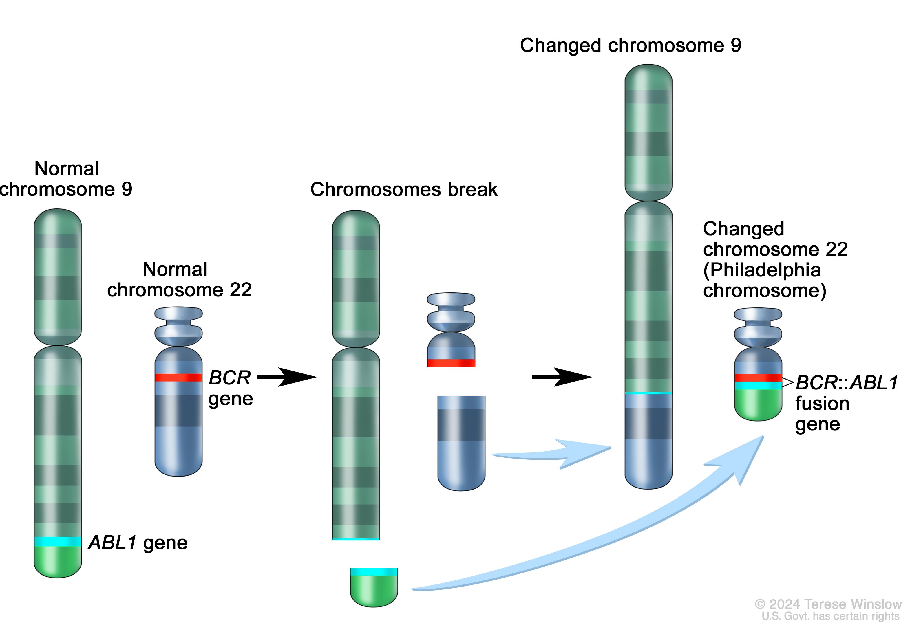
Famous Example
BCR-ABL fusion in CML(Chronic Myeloid Leukemia)
- discovered 1960
- translocation identified 1973
- imatinib approved 2001.
From observation to targeted therapy took 41 years; today we can do this computationally.
Exercises

Giphy