IGV and visualisation
Learning outcomes
After having completed this chapter you will be able to:
- Prepare a bam file for loading it into IGV
- Use IGV to:
- Navigate through a reference genome and alignments
- Retrieve information on a specific alignment
- Investigate (possible) variants
- Identify repeats and large INDELs
Material
Presentation on the UCSC genome browser (previous course):
Acknowledgement: the exercises below are partly based on this tutorial from the Griffith lab.
Exercises
A first glance: the E. coli dataset
Index the alignment that was filtered for the region between 2000 and 2500 kb:
cd ~/project/results/alignments
samtools index SRR519926.sorted.region.bam
SRR519926.sorted.region.bam) together with it’s index file (SRR519926.sorted.region.bam.bai) and the reference genome (ecoli-strK12-MG1655.fasta) to your desktop.
If working with Docker
If you are working with Docker, you can find the files in the working directory that you mounted to the docker container (with the -v option). So if you have used -v C:\Users\myusername\ngs-course:/root/project, your files will be in C:\Users\myusername\ngs-course.
- Load the genome (
.fasta) into IGV: Genomes > Load Genome from File… - Load the alignment file (
.bam): File > Load from File… -
Zoom in into the region U00096.3:2046000-2048000. You can do this in two ways:
- With the search box
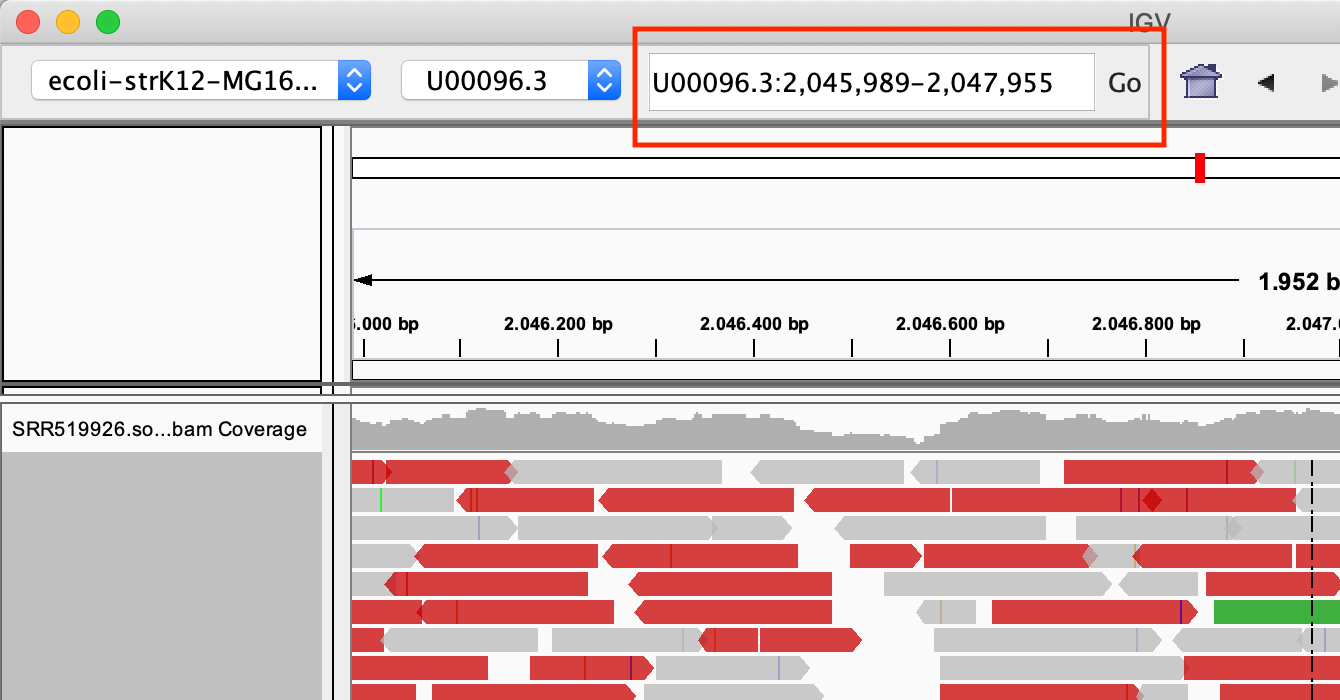
- Select the region in the location bar
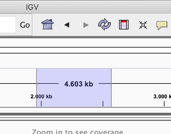
-
View the reads as pairs, by right click on the reads and select View as pairs
Exercise: There are lot of reads that are coloured red. Why is that?
If you don’t find any red reads..
The default setting is to color reads by insert size. However, if you’ve used IGV before, that might have changed. To color according to insert size: right click on the reads, and select: Color alignments by > insert size
Answer
According to IGV, reads are coloured red if the insert size is larger than expected. As you remember, this dataset has a very large variation in insert size.
Modify the popup text behaviour by clicking on the yellow balloon to Show Details on Click:
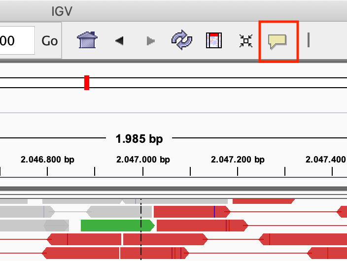
Exercise: Click on one of the reads. What kind of information is there?
Answer
Most of the information from the SAM file.
Colour the alignment by pair orientation by right clicking on the reads, and click Color alignments by > read strand.
HCC1143 data set
For this part, we will be using publicly available Illumina sequence data generated for the HCC1143 cell line. The HCC1143 cell line was generated from a 52 year old caucasian woman with breast cancer.
Sequence reads were aligned to version GRCh37 of the human reference genome. We will be working with subsets of aligned reads in the region: chromosome 21: 19,000,000 - 20,000,000.
The BAM files containing these reads for the cancer cell line and the matched normal are:
For these exercises, you can choose between IGV and the UCSC Genome Browser. Both tools have their strengths and weaknesses. IGV is a desktop application that you need to install on your computer, while the UCSC Genome Browser is web-based and runs in your browser.
If you choose IGV, download the BAM file and its index file to your computer. If you choose the UCSC Genome Browser, you don’t need to download any files, you can directly provide the URL to the BAM file.
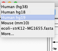
A lot of model-organism genomes are built-in IGV. Select the human genome version hg19 from the drop down menu:
Select File > Load from File… from the main menu and select the BAM file HCC1143.normal.21.19M-20M.bam using the file browser.
This BAM file only contains data for a 1 Megabase region of chromosome 21. Let’s navigate there to see what genes this region covers. To do so, navigate to chr21:19,000,000-20,000,000.
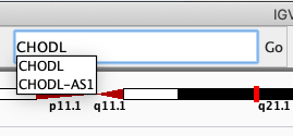
Navigate to the gene CHODL by typing it in the search box.
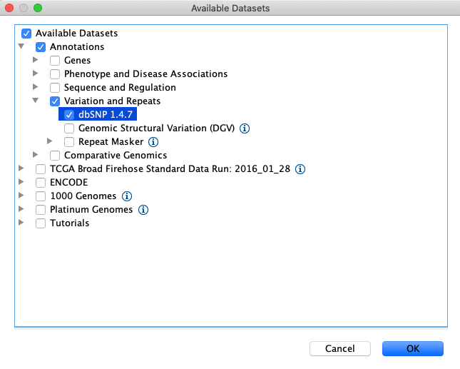
Load the dbsnp annotations by clicking File > Load From Server… > Annotations > Variation and Repeats > dbSNP 1.4.7
Like you did with the gene (i.e. by typing it in the search box), navigate to SNP rs3827160 that is annotated in the loaded file.
Click on the coverage track where the SNP is:
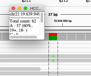
Exercise: What is the sequence sequencing depth for that base? And the percentage T?
Answer
The depth is 62, and 25 reads (40%) T.
Navigate to region chr21:19,800,320-19,818,162
Load repeat tracks by selecting File > Load from Server… from the main menu and then select Annotations > Variation and Repeats > Repeat Masker
Note
This might take a while to load.
Right click in the alignment track and select Color alignments by > insert size and pair orientation
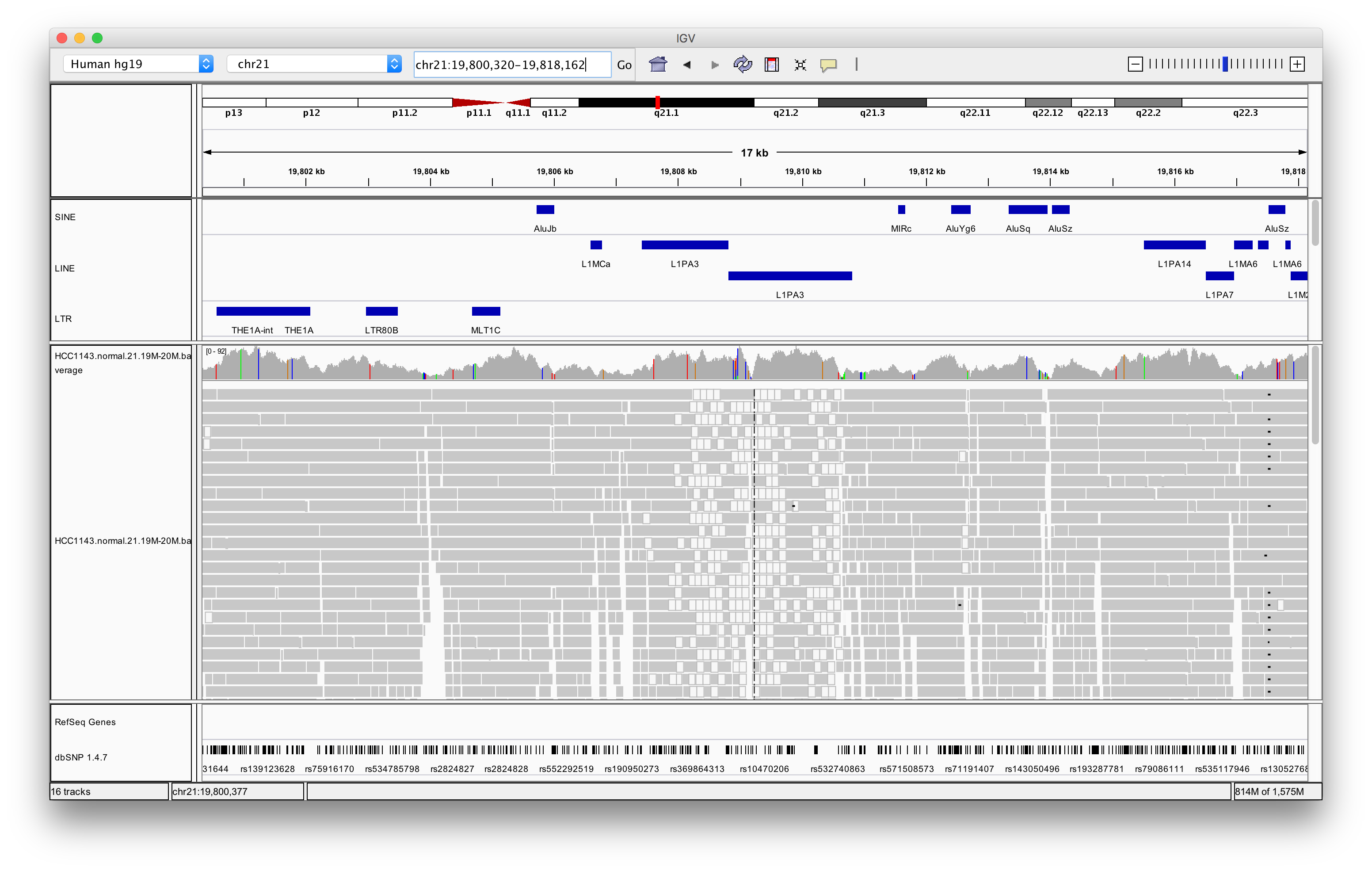
Exercise: Why are some reads coloured white? What can be the cause of that?
Answer
The white coloured reads have a map quality of 0 (click on the read to find the mapping quality). The cause of that is a LINE repeat region called L1PA3.
Navigate to region chr21:19,324,500-19,331,500
Right click in the main alignment track and select:
- Expanded
- View as pairs
- Color alignments by > insert size and pair orientation
- Sort alignments by > insert size
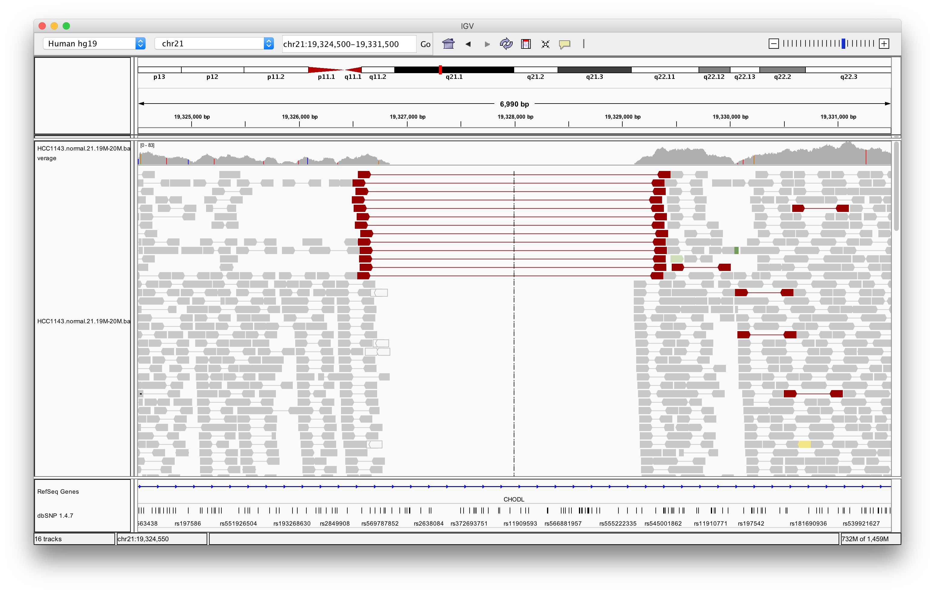
Exercise: What is the insert size of the red flagged read pairs? Can you estimate the size of the deletion?
Answer
The insert size is about 2.8 kb. This includes the reads. The deletion should be about 2.5 - 2.6 kb.
UCSC maintains and updates many genome assemblies and associated annotation data. The UCSC Genome Browser is web-based and runs in your browser. You can access it here: https://genome.ucsc.edu/.
Go to https://genome.ucsc.edu/. Click on Genomes in the top menu bar, and select Human GRCh37/hg19. This will open the genome browser for the human genome assembly GRCh37/hg19.

Our BAM file only contains data for a 1 Megabase region of chromosome 21. To load it, into the Genome Browser, we can directly provide the URL. For this, browse to My Data > Custom Tracks in the top menu bar.

This will open a menu where you can provide the URL to the BAM file. Paste the following URL into the text box at Paste URLs or data::
track type=bam name="HCC1143 normal" bigDataUrl=https://ngs-introduction-training.s3.eu-central-1.amazonaws.com/HCC1143.normal.21.19M-20M.bam pairEndsByName=.
Here we have specified that the file is of type BAM, given it a name (“HCC1143 normal”), and provided the URL to the BAM file. The option pairEndsByName=. specifies that the reads are paired-end and that the pairs can be identified by their names.
Note
Like IGV, the UCSC Genome Browser also needs the index file (.bai) to read the BAM file. The browser will automatically look for the index file in the same location as the BAM file, so you don’t need to provide it explicitly.
Click on Submit. This will add the BAM file as a custom track to your genome browser session. On the next page, click on Go to first annotation, which will take you to the location of the BAM file.
Let’s navigate there to see what genes this region covers. To do so, navigate to chr21:19,000,000-20,000,000. You can zoom in to any gene, but just typing the gene name in the search box. Type CHODL in the search box, and choose the entry you think represents are gene - this will take you to the gene location.
Like you did for the gene, navigate to SNP rs3827160.
Exercise: Is the individual homozygous or heterozygous for this variant?
Answer
We see both reference and alternate alleles, in an approximate 50/50 fashion, so the individual is most likely heterozygous.

Navigate to region chr21:19,800,320-19,818,162. After that, click on the track name or the gear icon to open the track settings. In the settings, select Use gray for and select alignment quality.
Exercise: Zoom in so you see the reads clearly. Why do some reads have a lighter color? To get alignment statistics for an individual read, click on it.
Answer
The light grey reads have a map quality of 0 (click on the read to find the mapping quality). The cause of that is a LINE repeat region called L1PA3. You can see this by checking the RepeatMasker track.
Navigate to region chr21:19,324,500-19,331,500. Make sure that you can see links between paired reads. You can enable this in the track settings by selecting Attempt to join paired end reads by name. In this region there is no coverage in the sample, indicating a homozygous deletion. What is the estimated insert size of the pairs that cover the region? Is that the true insert size? (Find it at Genomic size). Can you guess the size of the deletion by looking at the insert size of the reads spanning the deletion?
Answer

By clicking on one of the read pairs spanning the deletion, we can see that the insert size is about 2.8 kb. By looking at the coverage, we can estimate the deletion size to be about 2.4 - 2.5 kb.