Solution Step 2: Comparative Metagenome Analysis with SIAMCAT

General note: this guide has been written assuming you use a R.

Download the taxonomic profiles and metadata

Look at the metadata, how many controls (CTR) and cases (CRC for colorectal cancer) are there?

Solution

Load the data:

load(url("https://zenodo.org/record/6524317/files/motus_profiles_study1.Rdata"))

We can check what there is in the metadata with:

head(meta_study1)

There are many columns, but the one we are interesed in is "Group":

table(meta_study1$Group)

Which results in:

CRC CTR 
 46  60

There are 46 profiles from diseased patients (CRC) and 60 profiles from healthy individuals. We can check if there is an overall trend in the profiles looking at a PCA plot:

rel_ab = prop.table(motus_study1)
log_rel_ab = log10(rel_ab+ 10^-4)

# remove zero rows
log_rel_ab = log_rel_ab[rowSums(rel_ab) > 0,]

pc <- prcomp(t(log_rel_ab),
             center = TRUE,
             scale. = TRUE)

df = data.frame(
  pc1 = pc$x[,1],
  pc2 = pc$x[,2],
  Group = as.factor(meta_study1[rownames(pc$x),"Group"])
)

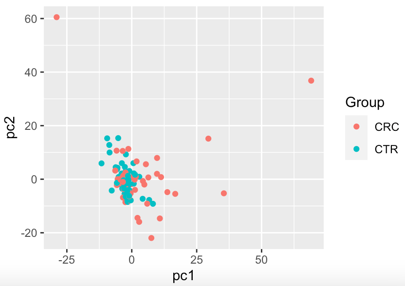
ggplot(df,aes(x = pc1,y = pc2, col = Group)) + geom_point()

Overall there is not a big shift visible from the PCA.

Identify which species show an association to colorectal cancer patients

Try to apply a t-test or a Wilcoxon test to your data.

Solution

Since we observed before that the data is not normally distributed, we can use a Wilcoxon test instead of a t-test. We can test all microbial species for statistically significant differences. In order to do so, we perform a Wilcoxon test on each individual bacterial species.

# use the same log transformed data as before
rel_ab = prop.table(motus_study1,2)
log_rel_ab = log10(rel_ab+ 10^-4)

# remove zero rows
log_rel_ab = log_rel_ab[rowSums(rel_ab) > 0,]

# we go through each measured species
p.vals <- rep_len(1, nrow(log_rel_ab))
names(p.vals) <- rownames(log_rel_ab)

for (i in rownames(log_rel_ab)){
  x <- log_rel_ab[i,]
  y <- meta_study1[colnames(log_rel_ab),]$Group
  t <- wilcox.test(x~y)
  p.vals[i] <- t$p.value
}
head(sort(p.vals))

Result:

                  Dialister pneumosintes [ref_mOTU_v3_03630] 
                                                1.277337e-07 
 Fusobacterium nucleatum subsp. animalis [ref_mOTU_v3_01001] 
                                                1.137605e-06 
           Olsenella sp. Marseille-P2300 [ref_mOTU_v3_10001] 
                                                2.184340e-05 
Fusobacterium nucleatum subsp. vincentii [ref_mOTU_v3_01002] 
                                                5.576030e-05 
          Anaerotignum lactatifermentans [ref_mOTU_v3_02190] 
                                                8.752588e-05 
Fusobacterium nucleatum subsp. nucleatum [ref_mOTU_v3_01003] 
                                                1.667614e-04

The species with the most significant effect seems to be Dialister pneumosintes, so let us take a look at the distribution of this species:

species <- 'Dialister pneumosintes [ref_mOTU_v3_03630]'
df.plot <- data.frame(
  log_rel_ab = log_rel_ab[species,],
  group = meta_study1[colnames(log_rel_ab),]$Group
)

ggplot(df.plot, aes(x=group, y=log_rel_ab)) +
  geom_boxplot(outlier.shape = NA) +
  geom_jitter(width = 0.08) + 
  xlab('') + 
  ylab('D. pneumosintes rel. ab. (log 10)')

Try to run SIAMCAT to do association testing.
Solution

We can also use the SIAMCAT R package to test for differential abundance and produce standard visualizations.
```
library("SIAMCAT")
```
Within SIAMCAT, the data are stored in the SIAMCAT object which contains the feature matrix, the metadata, and information about the groups you want to compare.
```
rel_ab = prop.table(motus_study1,2)
sc.obj <- siamcat(feat=rel_ab, meta=meta_study1, 
                  label='Group', case='CRC')
```
We can use SIAMCAT for feature filtering as well. Currently, the matrix of taxonomic profiles contains 33,571 different bacterial species. Of those, not all will be relevant for our question, since some are present only in a handful of samples (low prevalence) or at extremely low abundance. Therefore, it can make sense to filter your taxonomic profiles before you begin the analysis. Here, we could for example use the maximum species abundance as a filtering criterion. All species that have a relative abundance of at least 1e-03 in at least one of the samples will be kept, the rest is filtered out.
```
sc.obj <- filter.features(sc.obj, filter.method = 'abundance', cutoff = 1e-03)
```
Additionally we can filter based on the prevalence:
```
sc.obj <- filter.features(sc.obj, filter.method = 'prevalence', 
                          cutoff = 0.05, feature.type = 'filtered')
```
And we can have a look at the object:
```
sc.obj
```
Result:
```
siamcat-class object
label()                Label object:         60 CTR and 46 CRC samples
filt_feat()            Filtered features:    1167 features after abundance, prevalence filtering

contains phyloseq-class experiment-level object @phyloseq:
phyloseq@otu_table()   OTU Table:            [ 33571 taxa and 106 samples ]
phyloseq@sam_data()    Sample Data:          [ 106 samples by 12 sample variables ]
```
We go from 33,571 taxa to 1,167 after abundance and prevalence filtering.

Now, we can test the filtered feature for differential abundance with SIAMCAT:
```
sc.obj <- check.associations(sc.obj, detect.lim = 1e-05)
```

Build machine learning models to predict colorectal cancer patients from a metagenomic sample

Explore the SIAMCAT basic vignette to understand how you can train machine learning models to predict colerectal cancer from metagenomic samples.

The SIAMCAT machine learning workflow consists of several steps:
Normalization
SIAMCAT offers a few normalization approaches that can be useful for subsequent statistical modeling in the sense that they transform features in a way that can increase the accuracy of the resulting models. Importantly, these normalization techniques do not make use of any label information (patient status), and can thus be applied up front to the whole data set (and outside of the following cross validation).
```
sc.obj <- normalize.features(sc.obj, norm.method = 'log.std',
                             norm.param = list(log.n0=1e-05, sd.min.q=0))
# Features normalized successfully.
sc.obj
# siamcat-class object
# label()                Label object:         60 CTR and 46 CRC samples
# filt_feat()            Filtered features:    1167 features after abundance, prevalence filtering
# associations()         Associations:         Results from association testing
#                                              with 12 significant features at alpha 0.05
# norm_feat()            Normalized features:  1167 features normalized using log.std
# 
# contains phyloseq-class experiment-level object @phyloseq:
# phyloseq@otu_table()   OTU Table:            [ 33571 taxa and 106 samples ]
# phyloseq@sam_data()    Sample Data:          [ 106 samples by 12 sample variables ]
```
Cross Validation Split
Cross validation is a technique to assess how well an ML model would generalize to external data by partionining the dataset into training and test sets. Here, we split the dataset into 10 parts and then train a model on 9 of these parts and use the left-out part to test the model. The whole process is repeated 10 times.
```
sc.obj <- create.data.split(sc.obj, num.folds = 10, num.resample = 10)
# Features splitted for cross-validation successfully.
```
Model Training

Now, we can train a LASSO logistic regression classifier in order to distinguish CRC cases and controls.
```
sc.obj <- train.model(sc.obj, method='lasso')
# Trained lasso models successfully.
```
Predictions
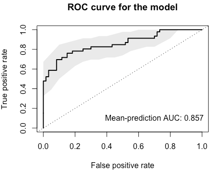
This function will automatically apply the models trained in cross validation to their respective test sets and aggregate the predictions across the whole data set.
```
sc.obj <- make.predictions(sc.obj)
# Made predictions successfully.
```
Model Evaluation
Calling the evaluate.predictions function will result in an assessment of precision and recall as well as in ROC analysis, both of which can be plotted:
```
sc.obj <- evaluate.predictions(sc.obj)
# Evaluated predictions successfully.
model.evaluation.plot(sc.obj)
```
ROC:

Precision-recall:
Model Interpretation

Finally, the model.interpretation.plot function will plot characteristics of the models (i.e. model coefficients or feature importance) alongside the input data aiding in understanding how / why the model works (or not).
```
model.interpretation.plot(sc.obj, consens.thres = 0.7)
```

Prediction on External Data

Apply the trained model (from study1_species.motus) on this new dataset and check the model performance on the external dataset. (Tip: Check out the help for the make.prediction function in SIAMCAT)

There are few steps:
Load the data

We load the data
```
load(url("https://zenodo.org/record/6524317/files/motus_profiles_study2.Rdata"))
```
And we create relative abundances:
```
rel_ab2 = prop.table(motus_study2,2)
```
Make predictions

We can now load the second dataset into a SIAMCAT object:
```
test.obj = siamcat(feat=rel_ab2, meta=meta_study2,
                   label='Group', case='CRC')
```
Now we can use the model that we built before (in sc.obj) and we can apply it to the test.obj holdout dataset. First, we will make the predictions on the based on the old dataset:
```
test.obj <- make.predictions(
siamcat = sc.obj,
siamcat.holdout = test.obj)
# note that the features are normalized with the same parameters for the old dataset

# evaluate the prediction
test.obj <- evaluate.predictions(test.obj)
```
Now, we can compare the performance of the classifier on the original and the holdout dataset by using the model.evaluation.plot function. Here, we can supply several SIAMCAT objects for which the model evaluation will be plotted in the same plot. Note that we can supply the objects as named objects in order to print the names in the legend.
```
model.evaluation.plot('Original' = sc.obj,
                      'Test' = test.obj ,
                       colours=c('dimgrey', 'orange'))
```