Glittr stats
In this report you can find some general statistics about Glittr.org. The plots and statistics created are amongst others used in the manuscript. Since Glittr.org is an ongoing project these statistics are updated weekly.
Set up the environment
This is required if you run this notebook locally. Loading required packages.
To run locally, create a file named .env and add your GitHub PAT (variable named PAT ) and google api key (named GOOGLE_API_KEY) in there, e.g.:
# this is an example, store it as .env:
export PAT="ghp_aRSRESCTZII20Lklser3H"
export GOOGLE_API_KEY="AjKSLE5SklxuRsxwPP8s0"
Now use your UNIX terminal to source this file to get the keys as objects:
source .envIn R, get environment variables as objects:
pat <- Sys.getenv("PAT")
google_api_key <- Sys.getenv("GOOGLE_API_KEY")
matomo_api_key <- Sys.getenv("MATOMO_API_KEY")
Setting colors. These correspond to the category colours on glittr.org.
glittr_cols <- c(
  "Scripting and languages" =             "#3a86ff",
  "Computational methods and pipelines" = "#fb5607",
  "Omics analysis" =                      "#ff006e",
  "Reproducibility and data management" = "#ffbe0b",
  "Statistics and machine learning" =     "#8338ec",
  "Others" =                              "#000000")
Parse repository data
Using the glittr.org REST API to get repository metadata, among which the stargazers, recency, category, license and tags.
Code
response <- request("https://glittr.org/api/repositories") |>
  req_perform() |>
  resp_body_json()

# extract relevant items as dataframe
repo_info_list <- lapply(response$data, function(x) {
  if(is.null(x$author$name)) {
    warning(sprintf("%s has no author specified", x$name))
  } else {
    data.frame(
    repo = x$name,
    author_name = x$author$name,
    stargazers = x$stargazers,
    recency = x$days_since_last_push,
    url = x$url,
    license = ifelse(is.null(x$license), "none", x$license),
    main_tag = x$tags[[1]]$name,
    main_category = x$tags[[1]]$category,
    website = x$website,
    author_profile = x$author$profile,
    author_website = x$author$website)
  }
})

repo_info <- do.call(rbind, repo_info_list)

# create a column with provider (either github or gitlab)
repo_info$provider <- ifelse(grepl("github", repo_info$url), "github", "gitlab")

# create a factor for categories for sorting
repo_info$main_category <- factor(repo_info$main_category,
                                  levels = names(glittr_cols))

# category table to keep order the same in the plots
cat_table <- table(category = repo_info$main_category)
cat_table <- sort(cat_table)
Number of repositories: 820
SIB courses not yet available on Glittr
Extracting course material URLs from the Bioschemas/JSON-LD markup on the SIB training materials page, then comparing those URLs with repository URLs that are already on Glittr.
Code
sib_request <- request("https://www.sib.swiss/training/training-materials")
sib_materials_page <- tryCatch(
sib_request |>
req_options(http_version = 2L) |>
req_perform() |>
resp_body_string(),
error = function(e) {
sib_request |>
req_options(http_version = 1L) |>
req_perform() |>
resp_body_string()
}
)
sib_doc <- read_html(sib_materials_page)
ld_json_blocks <- xml_find_all(sib_doc, "//script[@type='application/ld+json']") |>
xml_text(trim = TRUE)
is_course_node <- function(x) {
if(!is.list(x) || is.null(x$`@type`)) return(FALSE)
"Course" %in% as.character(x$`@type`)
}
collect_course_nodes <- function(x) {
out <- list()
if(is_course_node(x)) {
out <- c(out, list(x))
}
if(is.list(x)) {
for(el in x) {
out <- c(out, collect_course_nodes(el))
}
}
out
}
course_nodes <- list()
for(block in ld_json_blocks) {
parsed <- tryCatch(
jsonlite::fromJSON(block, simplifyVector = FALSE),
error = function(e) NULL
)
if(!is.null(parsed)) {
course_nodes <- c(course_nodes, collect_course_nodes(parsed))
}
}
extract_course_materials <- function(course) {
instances <- course$hasCourseInstance
if(is.null(instances)) return(NULL)
if(!is.list(instances) || (!is.null(instances$`@type`))) {
instances <- list(instances)
}
rows <- lapply(instances, function(instance) {
data.frame(
course = ifelse(is.null(course$name), NA, course$name),
course_instance_url = ifelse(is.null(instance$url), NA, instance$url),
material_url = ifelse(is.null(instance$workFeatured$url), NA,
instance$workFeatured$url),
stringsAsFactors = FALSE
)
})
do.call(rbind, rows)
}
course_materials <- lapply(course_nodes, extract_course_materials)
course_materials <- course_materials[!sapply(course_materials, is.null)]
course_materials <- do.call(rbind, course_materials)
course_materials <- course_materials |>
mutate(
material_url = gsub("&", "&", material_url, fixed = TRUE),
course_instance_url = gsub("&", "&", course_instance_url, fixed = TRUE)
) |>
distinct(course, material_url, .keep_all = TRUE)
normalize_repo_url <- function(url) {
if(is.na(url) || !nzchar(url)) return(NA_character_)
x <- trimws(tolower(url))
x <- gsub("&", "&", x, fixed = TRUE)
x <- sub("^https?://", "", x)
x <- sub("^www\\.", "", x)
x <- sub("\\?.*$", "", x)
x <- sub("#.*$", "", x)
x <- sub("/$", "", x)
x <- sub("\\.git$", "", x)
if(grepl("^[^/]+\\.github\\.io/", x)) {
parts <- strsplit(x, "/")[[1]]
org <- sub("\\.github\\.io$", "", parts[1])
repo <- if(length(parts) >= 2) parts[2] else NA_character_
if(!is.na(repo) && nzchar(repo)) {
x <- paste("github.com", org, repo, sep = "/")
}
}
if(grepl("^[^/]+\\.gitlab\\.io/", x)) {
parts <- strsplit(x, "/")[[1]]
group <- sub("\\.gitlab\\.io$", "", parts[1])
repo <- if(length(parts) >= 2) parts[2] else NA_character_
if(!is.na(repo) && nzchar(repo)) {
x <- paste("gitlab.com", group, repo, sep = "/")
}
}
if(grepl("^github\\.com/", x)) {
parts <- strsplit(x, "/")[[1]]
if(length(parts) >= 3) {
x <- paste(parts[1:3], collapse = "/")
}
}
if(grepl("^gitlab(\\.com|\\.sib\\.swiss)/", x)) {
x <- sub("/-/.+$", "", x)
parts <- strsplit(x, "/")[[1]]
if(length(parts) >= 3) {
x <- paste(parts[1:3], collapse = "/")
}
}
x
}
course_materials <- course_materials |>
mutate(material_key = sapply(material_url, normalize_repo_url))
course_materials_repo_like <- course_materials |>
filter(grepl("^(github\\.com|gitlab\\.com)/", material_key))
glittr_repo_keys <- unique(sapply(repo_info$url, normalize_repo_url))
missing_courses_on_glittr <- course_materials_repo_like |>
filter(!(material_key %in% glittr_repo_keys)) |>
distinct(course, material_key) |>
arrange(course)Number of SIB courses with repository-like materials not yet available on Glittr: 1
| course_title | material_key |
|---|---|
| Bonsai: Exploratory Analysis of Single-cell Data | github.com/ismara-unibas/bonsai_tutorial |
TeSS materials not yet available on Glittr
Using the TeSS API materials endpoint, extracting only resource links from GitHub/GitLab (including GitHub/GitLab Pages), and comparing those repositories with Glittr.
Code
tess_request <- request("https://tess.elixir-europe.org/materials") |>
  req_headers(Accept = "application/vnd.api+json")

fetch_tess_page <- function(page_number = 1, page_size = 200) {
  req <- tess_request |>
    req_url_query(page_number = page_number, page_size = page_size)

  resp <- tryCatch(
    req |>
      req_options(http_version = 2L) |>
      req_perform(),
    error = function(e) {
      req |>
        req_options(http_version = 1L) |>
        req_perform()
    }
  )

  resp_body_json(resp, simplifyVector = FALSE)
}

tess_pages <- list()
page_number <- 1
repeat {
  parsed <- fetch_tess_page(page_number = page_number, page_size = 200)
  tess_pages[[length(tess_pages) + 1]] <- parsed

  has_next <- !is.null(parsed$links$`next`)
  if(!has_next || length(parsed$data) == 0) break
  page_number <- page_number + 1
}

tess_materials <- do.call(c, lapply(tess_pages, function(x) x$data))

extract_tess_resource_urls <- function(material) {
  attrs <- material$attributes
  if(is.null(attrs)) return(character(0))

  urls <- c(
    attrs$url,
    attrs$doi
  )

  ext <- attrs[["external-resources"]]
  if(is.list(ext) && length(ext) > 0) {
    for(e in ext) {
      if(is.list(e) && !is.null(e$url)) {
        urls <- c(urls, e$url)
      } else if(is.character(e)) {
        urls <- c(urls, e)
      }
    }
  }

  urls <- urls[!is.na(urls) & nzchar(urls)]
  unique(urls)
}

tess_resources <- lapply(tess_materials, function(material) {
  attrs <- material$attributes
  urls <- extract_tess_resource_urls(material)

  if(length(urls) == 0) return(NULL)

  data.frame(
    material_title = ifelse(is.null(attrs$title), NA, attrs$title),
    tess_material_url = ifelse(is.null(material$links$self), NA,
                               paste0("https://tess.elixir-europe.org",
                                      material$links$self)),
    resource_url = urls,
    stringsAsFactors = FALSE
  )
})

tess_resources <- tess_resources[!sapply(tess_resources, is.null)]
tess_resources <- do.call(rbind, tess_resources)

tess_resources <- tess_resources |>
  mutate(resource_key = sapply(resource_url, normalize_repo_url)) |>
  filter(grepl("^(github\\.com|gitlab\\.com)/", resource_key))

tess_missing_on_glittr <- tess_resources |>
  filter(!(resource_key %in% glittr_repo_keys)) |>
  distinct(resource_key)
Number of TeSS materials with GitHub/GitLab resources not yet available on Glittr: 70
| repository |
|---|
| github.com/biocorecrg/rnaseq_coursescrg_2026 |
| github.com/biocorecrg/introduction-containers-course |
| github.com/ismara-unibas/bonsai_tutorial |
| github.com/elixir-cloud-aai/tutorials |
| github.com/vib-tcp/gentle-hands-on-python |
| github.com/marineomics/admin_03_panels.html |
| github.com/bgacademy23/easel-annotation |
| github.com/nadegeguiglielmoni/embo-24-genome-sequencing |
| github.com/ccgproject/ccgp_assembly |
| github.com/kamilsjaron/k-mer-approaches-for-biodiversity-genomics |
| github.com/524d/comparems2 |
| github.com/patterninstitute/osd758 |
| github.com/vib-tcp/genai_4_training-trainingmaterial |
| github.com/vib-tcp/functional_analysis_training |
| github.com/vib-tcp/containers-workshop |
| github.com/gtpb/am21 |
| github.com/pydna-group/pydna |
| github.com/hbctraining/intro-to-bulk-rnaseq |
| github.com/hbctraining/intro-to-scrnaseq |
| github.com/zemzemfiras1/nf-core-pre-hackathon_training2025 |
| github.com/hbctraining/tools-for-reproducible-research |
| github.com/hbctraining/intro-to-peak-analysis |
| github.com/hbctraining/intro-to-variant-analysis |
| github.com/hbctraining/shell-for-bioinformatics |
| github.com/hbctraining/investigating-chromatin-biology-chipseq |
| github.com/hbctraining/intro-to-dge |
| github.com/gallantries/video-library |
| github.com/elixirestonia/2024-11-06-git |
| github.com/biodata-pt/computational-tools-resources |
| github.com/gladstone-institutes/bioinformatics-presentations |
| github.com/elixir-europe-training/elixir-trp-fair-material-by-design |
| github.com/hds-sandbox/rdm_biodata_course |
| github.com/carpentries-incubator/fair-for-busy-biologists |
| github.com/sophie-a-lee/intro-rstudio-mhclg |
| github.com/carpentries-incubator/fair-research-software |
| github.com/sbwiecko/intuitive_biostatistics |
| github.com/mlabonne/blog |
| github.com/biologia-computacional/posts |
| github.com/nesper94/teaching |
| github.com/vibbits/rdm-introductory-course |
| github.com/ics80-fa21/website |
| github.com/liascript/course |
| github.com/mjfrigaard/shinypak |
| github.com/vibbits/nextflow-workshop |
| github.com/elixir-europe-training/elixir-trp-tess |
| gitlab.com/chrjan/seq-seq-pan |
| github.com/fairplus/fair_wizard |
| github.com/lcsb-biocore/cobrexa.jl |
| github.com/saezlab/cellnoptr |
| github.com/bridgedb/bridgedb-matlab |
| github.com/pathvisio/tutorials |
| github.com/dalalghamdi/ngbo |
| github.com/laurendupuis/scholia_tutorial |
| github.com/miappe/training |
| github.com/karrlab/de_sim |
| github.com/gtpb/3daroc18 |
| github.com/cbg-ethz/v-pipe |
| github.com/opencobra/cobratoolbox |
| github.com/openrisknet/workshop |
| github.com/eudat-training/b2safe-b2stage-training |
| github.com/uclouvain-cbio/bss2019 |
| github.com/enanomapper/tutorials |
| github.com/egonw/cdkbook |
| github.com/vjirsa/bootcamp |
| github.com/trainthetrainer/elixir-excelerate-ttt |
| github.com/nanocommons/tutorials |
| github.com/bigcat-um/bridgedbvariantdatabase |
| github.com/vdda/revealjs_test |
| github.com/swcarpentry/bc |
| github.com/datacarpentry/python-ecology |
Get contributors info
Using the GitHub REST API to get the number of contributors for each repository on glittr.org. This takes a few minutes, so if the contributors haven’t changed, it will use a cached version.
Code
# take long time to run, so try to use cache results if no repos have been
# added in the meantime

# check if data/n_contributors.rds exists
if(file.exists("data/n_contributors.rds")) {
  n_contributors <- readRDS("data/n_contributors.rds")
} else {
  n_contributors <- NULL
}

# get contributors info only from github repos
repo_info_gh <- repo_info[repo_info$provider == "github", ]

# get contributor info from github api if update is needed
if(!identical(sort(repo_info_gh$repo), sort(names(n_contributors)))) {
  dir.create("data", showWarnings = FALSE)
  n_contributors <- sapply(repo_info_gh$repo, function(x) {

    # get repo contributors
    resp <- request("https://api.github.com/repos/") |>
      req_url_path_append(x) |>
      req_url_path_append("contributors") |>
      req_url_query(per_page = 1) |>
      req_headers(
        Accept = "application/vnd.github+json",
        Authorization = paste("Bearer", pat),
        `X-GitHub-Api-Version` = "2022-11-28",
      ) |>
      req_perform()

    link_url <- resp_link_url(resp, "last")
    if(is.null(link_url)) {
      return(1)
    } else {
      npages <- strsplit(link_url, "&page=")[[1]][2] |> as.numeric()
      return(npages)
    }
  })

  # overwrite rds file
  saveRDS(n_contributors, "data/n_contributors.rds")
}

repo_info_gh$contributors <- n_contributors[repo_info_gh$repo]
Get country information
Here we get country information for all authors and organizations. It uses the free text specified at ‘location’. Since this can be anything, we use the google REST API to translate that into country.
Code
# check whether author info exists for caching
if(file.exists("data/author_info.rds")) {
  author_info <- readRDS("data/author_info.rds")
  author_info_authors <- unique(author_info$author) |> sort()
} else {
  author_info_authors <- NULL
}

gh_authors <- repo_info$author_name[repo_info$provider == "github"] |>
  unique() |>
  sort()

# if the author info is out of date, update it
if(!identical(gh_authors, author_info_authors)) {
  author_info_list <- list()
  for(author in gh_authors) {

    parsed <- request("https://api.github.com/users/") |>
      req_url_path_append(author) |>
      req_headers(
        Accept = "application/vnd.github+json",
        Authorization = paste("Bearer", pat),
        `X-GitHub-Api-Version` = "2022-11-28",
      ) |>
      req_perform() |>
      resp_body_json()

    author_info_list[[author]] <- data.frame(
      author = parsed$login,
      type = parsed$type,
      name = ifelse(is.null(parsed$name), NA, parsed$name),
      location = ifelse(is.null(parsed$location), NA, parsed$location)
    )
  }

  author_info <- do.call(rbind, author_info_list)

  author_info_loc <- author_info[!is.na(author_info$location), ]

  author_loc <- author_info_loc$location
  names(author_loc) <- author_info_loc$author

  ggmap::register_google(key = google_api_key)
  loc_info <- ggmap::geocode(author_loc,
                             output = 'all')

  get_country <- function(loc_results) {
    if("results" %in% names(loc_results)) {
      for(results in loc_results$results) {
        address_info <- results$address_components |>
          lapply(unlist) |>
          do.call(rbind, args = _) |>
          as.data.frame()
        country <- address_info$long_name[address_info$types1 == "country"]
        if (length(country) == 0) next
      }
      if (length(country) == 0) return(NA)
      return(country)
    } else {
      return(NA)
    }
  }

  countries <- sapply(loc_info, get_country)
  names(countries) <- names(author_loc)

  author_info$country <- countries[author_info$author]

  saveRDS(author_info, "data/author_info.rds")
}

repo_info <- merge(repo_info, author_info, by.x = "author_name",
                   by.y = "author")
repo_info$country[is.na(repo_info$country)] <- "undefined"- Number of authors: 369
- Number of countries: 30
Parse tag data
Here, we create tag_df that contains information for each tag by using the glittr.org API.
parsed <- request("https://glittr.org/api/tags") |>
  req_perform() |>
  resp_body_json()

tag_dfs <- list()
for(i in seq_along(parsed)) {
  category <- parsed[[i]]$category
  name <- sapply(parsed[[i]]$tags, function(x) x$name)
  repositories <- sapply(parsed[[i]]$tags, function(x) x$repositories)
  tag_dfs[[category]] <- data.frame(name, category, repositories)
}

tag_df <- do.call(rbind, tag_dfs) |> arrange(repositories)
Number of tags/topics: 67
Parse outlink data
Here, we use the matomo API to retrieve outlinks to repositories. In this way, we can have an idea which repositories are popular on glittr.org and how often people click on a link. It is summarized over a year (from today).
Code
url <- "https://matomo.sib.swiss/?module=API"

oneyearago <- format(Sys.Date() - 365, "%Y-%m-%d")

# Create and send the request
response <- request(url) |>
  req_body_form(
    method = "Actions.getOutlinks",
    idSite = 217,
    format = "json",
    date = paste(oneyearago, "today", sep = ","),
    period = "range",
    expanded = 1,
    filter_limit = -1,
    token_auth = matomo_api_key
  ) |>
  req_perform() |>
  resp_body_json()

## Get outlinks metadata in a dataframe
outlinks_list <- list()
for(domain in response) {
  label <- domain$label
  url_info <- lapply(domain$subtable, function(x) {
    data.frame(
      url = ifelse(is.null(x$url),NA , x$url),
      nb_visits = ifelse(is.null(x$nb_visits),NA , x$nb_visits),
      domain = label
    )
  })
  outlinks_list[[domain$label]] <- do.call(rbind, url_info)
}

outlinks_df <- do.call(rbind, outlinks_list)
row.names(outlinks_df) <- NULL

# function to clean urls for matching
clean_url <- function(url) {
  trimws(url) |> gsub("/$", "", x = _) |> tolower()
}

# function to match outlink data with repo and website url per entry
match_url <- function(outlinks_df, repo_info, column = "repo_url") {
  url_clean <- clean_url(outlinks_df$url)
  column_clean <- clean_url(repo_info[[column]])
  outlinks_df[[paste0("is_", column)]] <- url_clean %in% column_clean
  outlinks_df[[paste0("ass_repo_", column)]] <- repo_info$repo[match(url_clean,
                                                                    column_clean)]
  return(outlinks_df)
}

# apply the match url function on urls associated with repo entry
for(column in c("url", "website", "author_profile", "author_website")) {
  outlinks_df <- match_url(outlinks_df, repo_info, column = column)
}

# filter for only repo url and website (ignore author info)
# check whether associations match
outlinks_df$associated_entry <- outlinks_df |>
  select(ass_repo_url, ass_repo_website) |>
  apply(1, function(x) {
    x <- x[!is.na(x)] |> unique()

    if(length(x) == 1) return(x[1])
    if(length(x == 0) == 0) return(NA)
    if(length(x == 2)) return("do not correspond")
  })

# create a list of outlink visits by entry
visits_by_entry <- outlinks_df |>
  select(url, nb_visits, associated_entry) |>
  filter(!is.na(associated_entry)) |>
  group_by(associated_entry) |>
  summarise(total_visits = sum(nb_visits))

visits_by_entry <- merge(visits_by_entry, repo_info,
                         by.x = "associated_entry",
                         by.y = "repo") |>
  arrange(desc(total_visits))

visits_by_namespace <- visits_by_entry |>
  select(total_visits, author_name) |>
  group_by(author_name) |>
  summarise(total_visits = sum(total_visits)) |>
  arrange(desc(total_visits))

# visits by tag
visits_by_main_tag <- visits_by_entry |>
  select(total_visits, main_tag) |>
  group_by(main_tag) |>
  summarise(total_visits = sum(total_visits))

# add main category information for plotting
visits_by_main_tag <- merge(visits_by_main_tag, tag_df,
                            by.x = "main_tag",
                            by.y = "name") |>
  mutate(visits_per_repo = total_visits/repositories) |>
arrange(desc(visits_per_repo))- The number of outlink visits in the last year: 2193
- Number of repositories found using Glittr.org: 232
- Most popular repo was TheAlgorithms/Python with 224 outlinks.
- Most popular namespace was TheAlgorithms with 224 outlinks.
Number of repositories by category
This is figure 2A in the manuscript.
cat_count_plot <- table(category = repo_info$main_category) |>
  as.data.frame() |>
  ggplot(aes(x = reorder(category, Freq), y = Freq, fill = category)) +
  geom_bar(stat = "identity") +
  scale_fill_manual(values = glittr_cols) +
  coord_flip() +
  theme_classic() +
  ggtitle("Categories") +
  theme(legend.position = "none",
        axis.title.y = element_blank()) +
  ylab("Number of repositories")

print(cat_count_plot)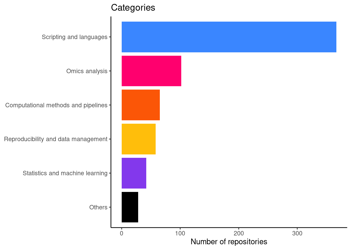
And a table with the actual numbers
category_count <- table(category = repo_info$main_category) |> as.data.frame()
knitr::kable(category_count)| category | Freq |
|---|---|
| Scripting and languages | 343 |
| Computational methods and pipelines | 56 |
| Omics analysis | 221 |
| Reproducibility and data management | 61 |
| Statistics and machine learning | 105 |
| Others | 32 |
Number of contributors per repository separated by category
This is figure 2B in the manuscript.
repo_info_gh$main_category <- factor(repo_info_gh$main_category,
                                     levels = names(cat_table))

contributors_plot <- repo_info_gh |>
  ggplot(aes(x = main_category, y = contributors, fill = main_category)) +
  geom_violin(scale = "width") +
  geom_boxplot(width = 0.1, col = "darkgrey") +
  coord_flip() +
  ggtitle("Contributors") +
  ylab("Number of contributors") +
  scale_y_sqrt() +
  scale_fill_manual(values = glittr_cols) +
  theme_bw() +
  theme(legend.position = "none",
        axis.title.y = element_blank(),
        plot.margin = margin(t = 5, r = 10, b = 5, l = 10))

print(contributors_plot)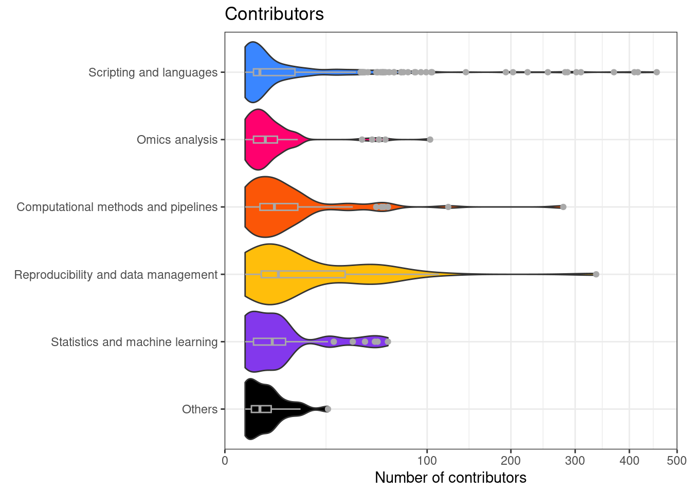
And some statistics of contributors.
- More than 10 contributors: 23.7%
- More than 1 contributor: 78.6%
- Between 1 and 5 contributors: 62.1%
Number of repositories per tag
This is figure 2C in the manuscript.
tag_freq_plot <- tag_df |>
  filter(repositories > 10) |>
  ggplot(aes(x = reorder(name, repositories),
             y = repositories, fill = category)) +
  geom_bar(stat = "identity") +
  coord_flip() +
  scale_fill_manual(values = glittr_cols) +
  ggtitle("Tags with > 10 repositories") +
  ylab("Number of repositories") +
  annotate(geom = "text", x = 2, y = 150,
           label = paste("Total number of tags: ",
                         nrow(tag_df)),
           color="black") +
  theme_classic() +
  theme(legend.position = "none",
        axis.title.y = element_blank())

print(tag_freq_plot)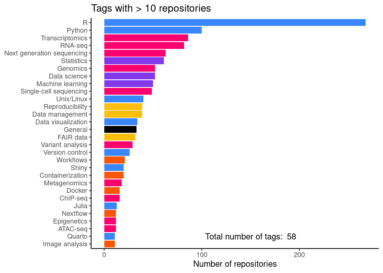
And a table with the actual numbers.
Number of repositories by author
This is figure 2D in the manuscript.
author_freq <- table(author_name = repo_info$author_name,
                     main_category = repo_info$main_category) |>
  as.data.frame()

author_freq$main_category <- factor(author_freq$main_category,
                                     levels = names(cat_table))

repos_per_author <- table(repo_info$author_name)

lf_authors <- names(repos_per_author)[repos_per_author < 5]

author_freq_plot <- author_freq |>
  filter(!author_name %in% lf_authors) |>
  arrange(Freq) |>
  ggplot(aes(x = reorder(author_name, Freq), y = Freq, fill = main_category)) +
  geom_bar(stat = "identity") +
  coord_flip() +
  ggtitle("Author or organization") +
  ylab("Number of repositories") +
  scale_fill_manual(values = glittr_cols) +
  annotate(geom = "text", x = 2, y = 30,
           label = paste("Authors with < 5 repos: ",
                         length(lf_authors)),
           color="black") +
  theme_classic() +
  theme(legend.position = "none",
        axis.title.y = element_blank())

print(author_freq_plot)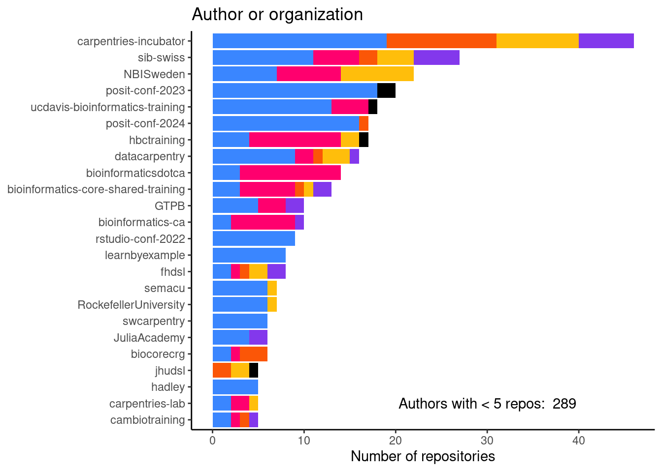
And a table with the actual numbers.
Number of repositories per license
This is figure 2E in the manuscript.
lic_freq_data <- table(license = repo_info$license,
                       main_category = repo_info$main_category) |>
  as.data.frame()

lic_freq_data$main_category <- factor(lic_freq_data$main_category,
                                     levels = names(cat_table))

lic_freq_plot <- lic_freq_data |>
  ggplot(aes(x = reorder(license, Freq), y = Freq, fill = main_category)) +
  geom_bar(stat = "identity") +
  coord_flip() +
  scale_fill_manual(values = glittr_cols) +
  theme_classic() +
  ggtitle("License type") +
  ylab("Number of repositories") +
  theme(legend.position = "none",
        axis.title.y = element_blank())

print(lic_freq_plot)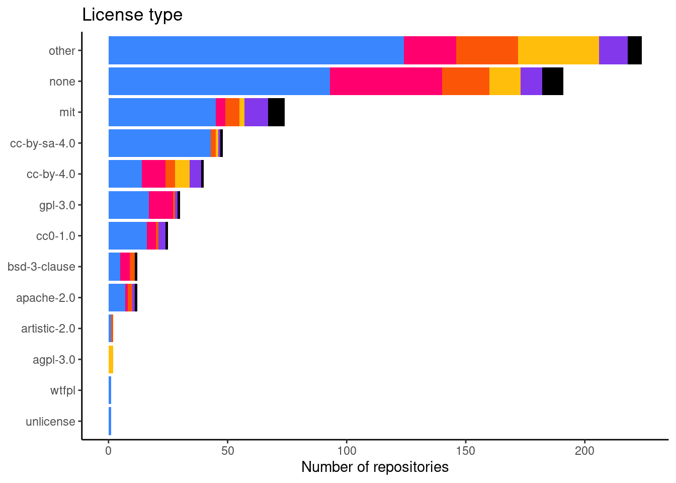
And a table with the actual numbers.
| Var1 | Freq | perc |
|---|---|---|
| other | 262 | 32.0 |
| none | 242 | 29.6 |
| mit | 96 | 11.7 |
| cc-by-4.0 | 73 | 8.9 |
| cc-by-sa-4.0 | 51 | 6.2 |
| gpl-3.0 | 34 | 4.2 |
| cc0-1.0 | 28 | 3.4 |
| bsd-3-clause | 14 | 1.7 |
| apache-2.0 | 12 | 1.5 |
| agpl-3.0 | 2 | 0.2 |
| artistic-2.0 | 2 | 0.2 |
| unlicense | 1 | 0.1 |
| wtfpl | 1 | 0.1 |
Number of repositories per country
This is figure 2F in the mansucript.
country_freq <- table(country = repo_info$country,
                      main_category = repo_info$main_category) |>
  as.data.frame()

country_freq$main_category <- factor(country_freq$main_category,
                                     levels = names(cat_table))

country_freq_plot <- country_freq |>
  filter(country != "undefined") |>
  ggplot(aes(x = reorder(country, Freq), y = Freq, fill = main_category)) +
  geom_bar(stat = "identity") +
  coord_flip() +
  ggtitle("Country") +
  ylab("Number of repositories") +
  scale_fill_manual(values = glittr_cols) +
  annotate(geom = "text", x = 2, y = 70,
           label = paste("Repos with undefined country: ",
                         sum(repo_info$country == "undefined")),
           color="black") +
  theme_classic() +
  theme(legend.position = "none",
        axis.title.y = element_blank())

print(country_freq_plot)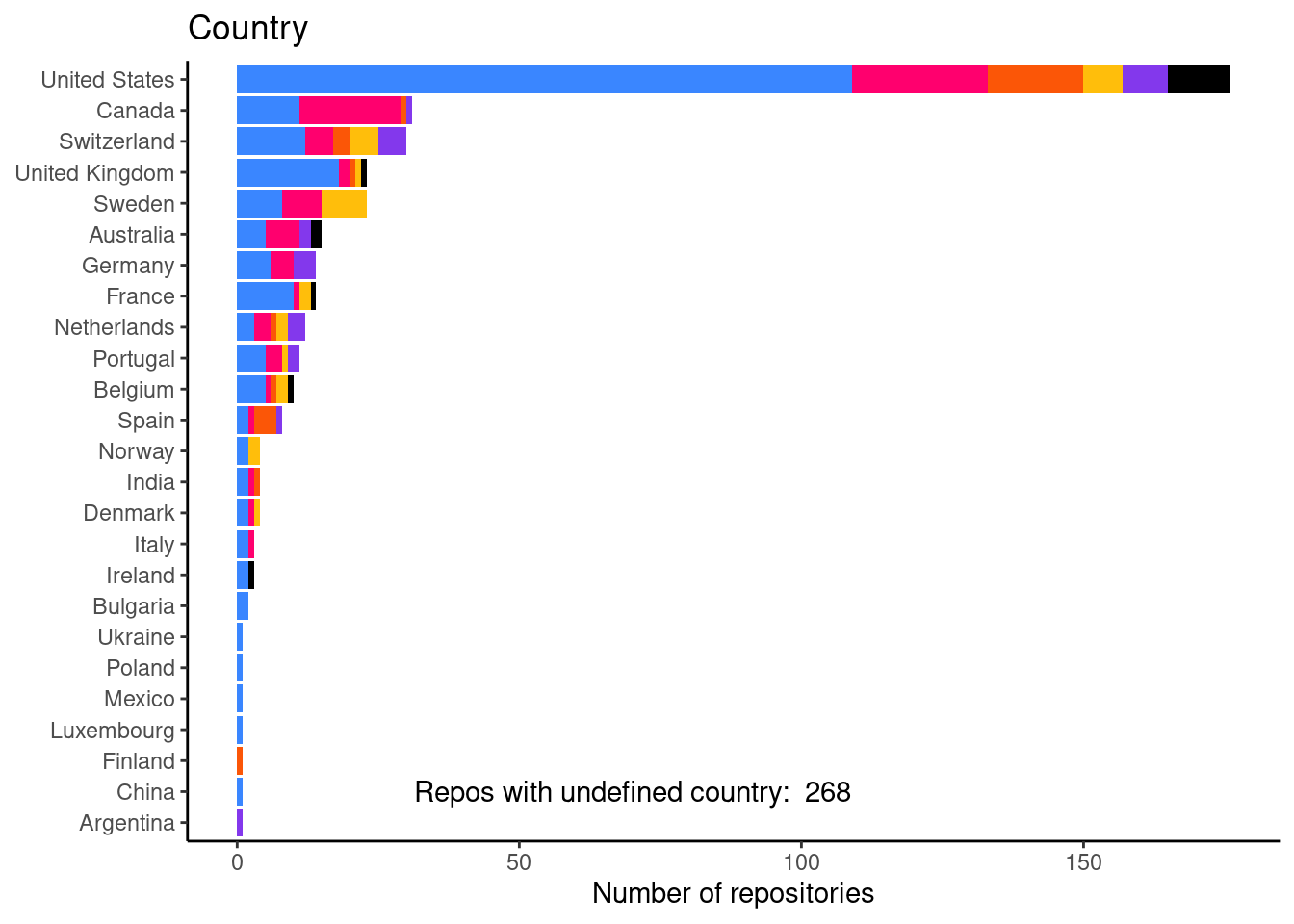
And a table with the actual numbers.
repo_info$country |>
  table() |>
  as.data.frame() |>
  arrange(desc(Freq)) |>
knitr::kable()| Var1 | Freq |
|---|---|
| undefined | 323 |
| United States | 196 |
| Canada | 53 |
| Switzerland | 51 |
| United Kingdom | 30 |
| Sweden | 26 |
| Portugal | 20 |
| Australia | 18 |
| Germany | 18 |
| Belgium | 15 |
| Netherlands | 14 |
| France | 13 |
| Spain | 9 |
| Denmark | 5 |
| India | 4 |
| Norway | 4 |
| Italy | 3 |
| Bulgaria | 2 |
| Ireland | 2 |
| Luxembourg | 2 |
| Argentina | 1 |
| China | 1 |
| Czechia | 1 |
| Estonia | 1 |
| Finland | 1 |
| Mexico | 1 |
| New Zealand | 1 |
| Poland | 1 |
| South Africa | 1 |
| Ukraine | 1 |
Number of outlinks by repo
Here, we use the site data from matomo in order to investigate what visitors of Glittr.org have clicked on. This gives us an idea about which repositories and topics are popular among users. In Figure 7 we see that TheAlgorithms/Python was the most popular repository with 224 clicks.
visits_by_entry |>
  slice(1:30) |>
  ggplot(aes(x = reorder(associated_entry, total_visits),
             y = total_visits, fill = main_category)) +
  geom_bar(stat = "identity") +
  coord_flip() +
  scale_fill_manual(values = glittr_cols) +
  ggtitle("Top 30 of most outlinked repos") +
  ylab("Number of outlinks") +
  theme_classic() +
  theme(legend.position = "none",
        axis.title.y = element_blank())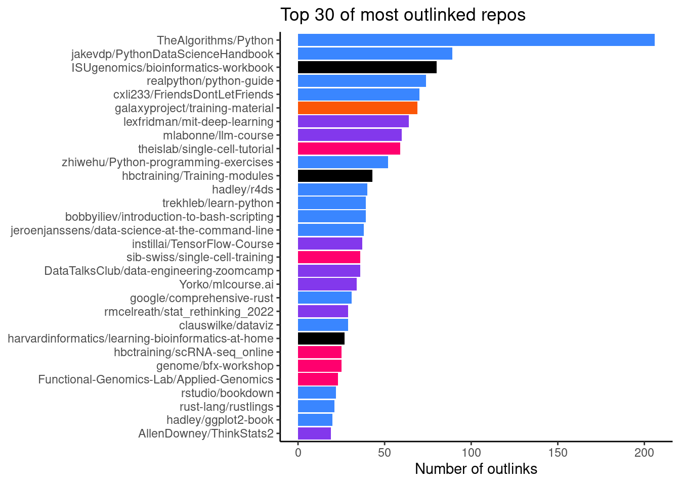
| repository | total_visits |
|---|---|
| TheAlgorithms/Python | 224 |
| mlabonne/llm-course | 81 |
| jakevdp/PythonDataScienceHandbook | 67 |
| ISUgenomics/bioinformatics-workbook | 64 |
| gladstone-institutes/Bioinformatics-Workshops | 62 |
| galaxyproject/training-material | 56 |
| hbctraining/Intro-to-scRNAseq | 48 |
| theislab/single-cell-tutorial | 48 |
| realpython/python-guide | 42 |
| bobbyiliev/introduction-to-bash-scripting | 41 |
| cxli233/FriendsDontLetFriends | 38 |
| pachterlab/BI-BE-CS-183-2023 | 37 |
| hadley/r4ds | 35 |
| sib-swiss/single-cell-training | 32 |
| zhiwehu/Python-programming-exercises | 30 |
| rust-lang/rustlings | 29 |
| DataTalksClub/data-engineering-zoomcamp | 28 |
| hbctraining/Training-modules | 28 |
| hbctraining/Intro-to-bulk-RNAseq | 26 |
| theislab/single-cell-best-practices | 26 |
| harvardinformatics/learning-bioinformatics-at-home | 25 |
| trekhleb/learn-python | 25 |
| lexfridman/mit-deep-learning | 24 |
| telatin/microbiome-bioinformatics | 24 |
| griffithlab/rnabio.org | 23 |
| biotrain-latam/BiotrAIn-pilot-course | 22 |
| Yorko/mlcourse.ai | 22 |
| Graylab/DL4Proteins-notebooks | 21 |
| sib-swiss/spatial-transcriptomics-training | 21 |
| raphaelmourad/LLM-for-genomics-training | 20 |
It becomes more interesting when we aggregate the data per main tag (Figure 8). This gives us an idea of topic which people are looking for when visiting glittr.org. The most popular topic is Python with 458 outlinks.
visits_by_main_tag |>
  slice(1:30) |>
  ggplot(aes(x = reorder(main_tag, total_visits),
             y = total_visits, fill = category)) +
  geom_bar(stat = "identity") +
  coord_flip() +
  scale_fill_manual(values = glittr_cols) +
  ggtitle("Top 30 of most outlinked main tags") +
  ylab("Number of outlinks") +
  theme_classic() +
  theme(legend.position = "none",
        axis.title.y = element_blank())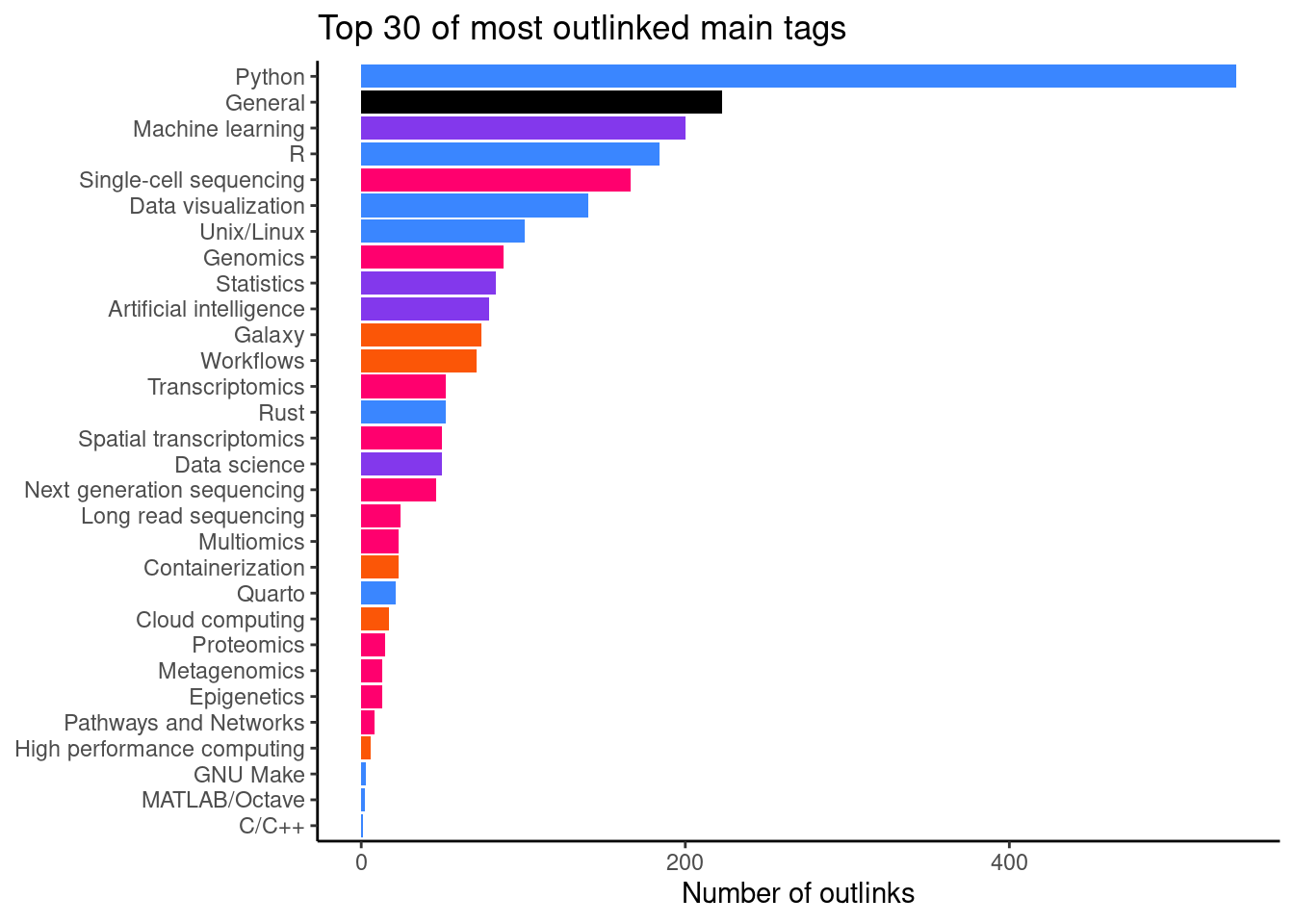
When we normalize the visits by number of repositories per tag (Figure 9), we can get an idea where training materials might be lacking. A high number here show repositories that are quite unique in what they teach, but are still popular. Here, we see that there are 4 repositires with the main tag Large language models with an average of 25.5 outlinks.
visits_by_main_tag |>
  arrange(desc(visits_per_repo)) |>
  slice(1:30) |>
  ggplot(aes(x = reorder(main_tag, visits_per_repo),
             y = visits_per_repo, fill = category)) +
  geom_bar(stat = "identity") +
  coord_flip() +
  scale_fill_manual(values = glittr_cols) +
  ggtitle("Top 30 of most outlinked main tags normalized by repo number") +
  ylab("Number of outlinks per tag/number of repositories having tag") +
  theme_classic() +
  theme(legend.position = "none",
        axis.title.y = element_blank())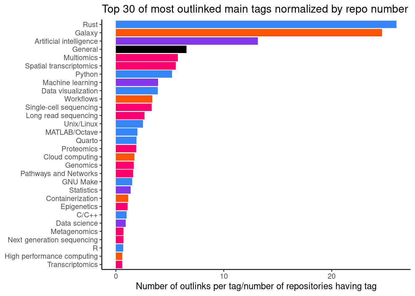
| main_tag | total_visits | category | repositories | visits_per_repo |
|---|---|---|---|---|
| Large language models | 102 | Statistics and machine learning | 4 | 25.5000000 |
| Rust | 41 | Scripting and languages | 2 | 20.5000000 |
| Protein structure | 21 | Omics analysis | 2 | 10.5000000 |
| Galaxy | 56 | Computational methods and pipelines | 6 | 9.3333333 |
| General | 310 | Others | 37 | 8.3783784 |
| Single-cell sequencing | 231 | Omics analysis | 59 | 3.9152542 |
| Python | 458 | Scripting and languages | 120 | 3.8166667 |
| Unix/Linux | 110 | Scripting and languages | 49 | 2.2448980 |
| Multiomics | 19 | Omics analysis | 9 | 2.1111111 |
| Data visualization | 92 | Scripting and languages | 44 | 2.0909091 |
| Spatial transcriptomics | 41 | Omics analysis | 20 | 2.0500000 |
| LaTeX | 2 | Scripting and languages | 1 | 2.0000000 |
| Artificial intelligence | 29 | Statistics and machine learning | 15 | 1.9333333 |
| Proteomics | 18 | Omics analysis | 10 | 1.8000000 |
| Machine learning | 91 | Statistics and machine learning | 63 | 1.4444444 |
| Epigenetics | 16 | Omics analysis | 12 | 1.3333333 |
| Metagenomics | 32 | Omics analysis | 24 | 1.3333333 |
| Workflows | 31 | Computational methods and pipelines | 24 | 1.2916667 |
| GNU Make | 3 | Scripting and languages | 3 | 1.0000000 |
| Metabolomics | 5 | Omics analysis | 5 | 1.0000000 |
| High performance computing | 12 | Computational methods and pipelines | 14 | 0.8571429 |
| Transcriptomics | 91 | Omics analysis | 107 | 0.8504673 |
| Statistics | 49 | Statistics and machine learning | 71 | 0.6901408 |
| Genomics | 52 | Omics analysis | 77 | 0.6753247 |
| Variant analysis | 23 | Omics analysis | 38 | 0.6052632 |
| Long read sequencing | 8 | Omics analysis | 14 | 0.5714286 |
| Data science | 33 | Statistics and machine learning | 64 | 0.5156250 |
| Next generation sequencing | 38 | Omics analysis | 92 | 0.4130435 |
| R | 122 | Scripting and languages | 296 | 0.4121622 |
| Java | 1 | Scripting and languages | 3 | 0.3333333 |
We can also check popularity by namespace, i.e. author (Table 10).
| author_name | total_visits |
|---|---|
| TheAlgorithms | 224 |
| sib-swiss | 168 |
| hbctraining | 125 |
| mlabonne | 81 |
| NBISweden | 74 |
| theislab | 74 |
| jakevdp | 67 |
| ISUgenomics | 64 |
| gladstone-institutes | 62 |
| hadley | 60 |
| galaxyproject | 56 |
| realpython | 42 |
| bobbyiliev | 41 |
| cxli233 | 38 |
| pachterlab | 37 |
| griffithlab | 31 |
| carpentries-incubator | 30 |
| zhiwehu | 30 |
| rust-lang | 29 |
| DataTalksClub | 28 |
| harvardinformatics | 25 |
| trekhleb | 25 |
| lexfridman | 24 |
| telatin | 24 |
| Yorko | 22 |
| biotrain-latam | 22 |
| Graylab | 21 |
| carpentries-lab | 21 |
| UCLouvain-CBIO | 20 |
| raphaelmourad | 20 |
Summary plot
Full figure 2 of the manuscript.