QC and alignment
Learning outcomes
After having completed this chapter you will be able to:
- Explain how the fastq format stores sequence and base quality information and why this is limited for long-read sequencing data
- Calculate base accuracy and probability based on base quality
- Describe how alignment information is stored in a sequence alignment (
.sam) file - Perform a quality control on long-read data with
NanoPlot - Perform a basic alignment of long reads with
minimap2 - Visualise an alignment file in IGV on a local computer
Material
Exercises
1. Retrieve data
We will be working with data from:
Padilla, Juan-Carlos A., Seda Barutcu, Ludovic Malet, Gabrielle Deschamps-Francoeur, Virginie Calderon, Eunjeong Kwon, and Eric Lécuyer. “Profiling the Polyadenylated Transcriptome of Extracellular Vesicles with Long-Read Nanopore Sequencing.” BMC Genomics 24, no. 1 (September 22, 2023): 564. https://doi.org/10.1186/s12864-023-09552-6.
The authors used RNA sequencing with Oxford Nanopore Technology of both extracellular vesicles and whole cells from cell culture.
For the exercises of today, we will work with two samples of this study. Download and unpack the data files in your home directory.
cd ~/project
wget https://ngs-longreads-training.s3.eu-central-1.amazonaws.com/project1.tar.gz
tar -xvf project1.tar.gz
rm project1.tar.gz
Exercise: This will create the directory called project1. Check out what’s in there.
Answer
Go to the ~/project/project1 folder:
cd ~/project/project1
The data folder contains the following:
project1/
├── reads
│   ├── Cell_1.fastq.gz
│   ├── Cell_2.fastq.gz
│   ├── Cell_3.fastq.gz
│   ├── EV_1.fastq.gz
│   ├── EV_2.fastq.gz
│   └── EV_3.fastq.gz
├── reads_manifest.tsv
└── references
    ├── Homo_sapiens.GRCh38.111.chr5.chr6.chrX.gtf
    └── Homo_sapiens.GRCh38.dna.primary_assembly.chr5.chr6.chrX.fa

2 directories, 9 files
reads_manifest.csv. EV means ‘extracellular vesicle’, Cell means ‘entire cells’. In the references folder you can find the reference sequence and annotation.
2. Quality control
Activate the conda environment
The tools you will be needed for these exercises are in the conda environment lr-tools. Every time you open a new terminal, activate it with:
conda activate lr-tools
We will evaluate the read quality of two fastq files with NanoPlot.
Exercise: Check out the manual of NanoPlot with the command NanoPlot --help. After that run NanoPlot on
reads/Cell_2.fastq.gzreads/EV_2.fastq.gz.
Your fastq files are in the ‘rich’ format, meaning they have additional information regarding the ONT run.
Hint
For a basic output of NanoPlot on a fastq.gz file you can use the options --outdir and --fastq_rich.
Answer
We have a rich fastq file, so based on the manual and the example we can run:
cd ~/project/project1

mkdir -p nanoplot

NanoPlot \
--fastq_rich reads/Cell_2.fastq.gz \
--outdir nanoplot/Cell_2

NanoPlot \
--fastq_rich reads/EV_2.fastq.gz \
--outdir nanoplot/EV_2
In both directories you will now have a directory with the following files:
.
├── ActivePores_Over_Time.html
├── ActivePores_Over_Time.png
├── ActivityMap_ReadsPerChannel.html
├── ActivityMap_ReadsPerChannel.png
├── CumulativeYieldPlot_Gigabases.html
├── CumulativeYieldPlot_Gigabases.png
├── CumulativeYieldPlot_NumberOfReads.html
├── CumulativeYieldPlot_NumberOfReads.png
├── LengthvsQualityScatterPlot_dot.html
├── LengthvsQualityScatterPlot_dot.png
├── LengthvsQualityScatterPlot_kde.html
├── LengthvsQualityScatterPlot_kde.png
├── NanoPlot_20240221_1219.log
├── NanoPlot-report.html
├── NanoStats.txt
├── Non_weightedHistogramReadlength.html
├── Non_weightedHistogramReadlength.png
├── Non_weightedLogTransformed_HistogramReadlength.html
├── Non_weightedLogTransformed_HistogramReadlength.png
├── NumberOfReads_Over_Time.html
├── NumberOfReads_Over_Time.png
├── TimeLengthViolinPlot.html
├── TimeLengthViolinPlot.png
├── TimeQualityViolinPlot.html
├── TimeQualityViolinPlot.png
├── WeightedHistogramReadlength.html
├── WeightedHistogramReadlength.png
├── WeightedLogTransformed_HistogramReadlength.html
├── WeightedLogTransformed_HistogramReadlength.png
├── Yield_By_Length.html
└── Yield_By_Length.png

0 directories, 31 files
The file NanoPlot-report.html contains a report with all the information stored in the other files, and NanoStats.txt in text format.
Exercise: Check out some of the .png plots and the contents of NanoStats.txt. Also, download NanoPlot-report.html for both files to your local computer and answer the following questions:
A. How many reads are in the files?
B. What are the average read lengths? What does this tell us about the quality of both runs?
C. What is the average base quality and what kind of accuracy do we therefore expect?
D. Browse through the report and check out the other plots. Was there a site dependency in the number of reads per channel? Would a longer sequencing run have been beneficial?
Download files from the notebook
You can download files from the file browser, by right-clicking a file and selecting Download…:
Answer
A. Cell_2: 49,808 reads; EV_2: 6,214 reads
B. Cell_2: 1186.7 EV_2: 607.9. Both runs are form cDNA. Transcripts are usually around 1-2kb. The average read length is therefore quite short in sample EV_2.
C. The median base quality is for both around 12. This means that the error probability is about 10^(-12/10) = 0.06, so an accuracy of 94%.
D. The number of reads per channel is variable (check out ‘Number of reads generated per channel’). There is a spot in the middle of the flow cell with channels with very low activity. Both the cumulative yield plots and the number of reads over time plots show that the run was reaching saturation. A longer run would not have been beneficial.
3. Read alignment
The sequence aligner minimap2 is specifically developed for (splice-aware) alignment of long reads.
Exercise: Checkout the helper minimap2 --help and/or the github readme. We are working with reads generated from cDNA. Considering we are aligning to a reference genome (DNA), what would be the most logical parameter for our dataset to the option -x?
Answer
The option -x can take the following arguments:
-x STR       preset (always applied before other options; see minimap2.1 for details) []
           - map-pb/map-ont: PacBio/Nanopore vs reference mapping
           - ava-pb/ava-ont: PacBio/Nanopore read overlap
           - asm5/asm10/asm20: asm-to-ref mapping, for ~0.1/1/5% sequence divergence
           - splice: long-read spliced alignment
           - sr: genomic short-read mapping
map-ont. However, our data is also spliced. Therefore, we should choose splice.
Exercise: Make a directory called alignments in your working directory. After that, modify the command below for minimap2 and run it from a script; i.e. replace [PARAMETER] with the correct option.
#!/usr/bin/env bash

cd ~/project/project1

mkdir -p alignments

for sample in EV_2 Cell_2; do
    minimap2 \
    -a \
    -x [PARAMETER] \
    -t 4 \
    references/Homo_sapiens.GRCh38.dna.primary_assembly.chr5.chr6.chrX.fa \
    reads/"$sample".fastq.gz \
    | samtools sort \
    | samtools view -bh > alignments/"$sample".bam

    ## indexing for IGV
    samtools index alignments/"$sample".bam
done
Note
Once your script is running, it will take a while to finish. Have a ☕.
Answer
Modify the script to set the -x option:
#!/usr/bin/env bash

cd ~/project/project1

mkdir -p alignments

for sample in EV_2 Cell_2; do
    minimap2 \
    -a \
    -x splice \
    -t 4 \
    references/Homo_sapiens.GRCh38.dna.primary_assembly.chr5.chr6.chrX.fa \
    reads/"$sample".fastq.gz \
    | samtools sort \
    | samtools view -bh > alignments/"$sample".bam

    ## indexing for IGV
    samtools index alignments/"$sample".bam
done
And run it (e.g. if you named the script ont_alignment.sh):
chmod u+x ont_alignment.sh
./ont_alignment.sh
4. Visualisation
Let’s have a look at the alignments. Download the files (in ~/project/project1/alignments):
EV_2.bamEV_2.bam.baiCell_2.bamCell_2.bam.bai
to your local computer and load the .bam files into IGV (File > Load from File…).
Exercise: Have a look at the gene ELOVL5 by typing the name into the search box.
- Do you see any evidence for alternative splicing already?
- How is the difference in quality between the two samples? Would that have an effect on estimating differential splicing?
Check out the paper
The authors found splice variants. Check figure 5B in the paper.
Answer
There is some observable exon skipping in Cell_2:
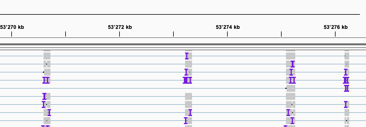
The coverage of EV_2 is quite low. Also, a lot of the reads do not fully cover the gene. This will make it difficult to estimate differential splicing.