library(Seurat)
library(ggplot2)
library(clustree)
library(patchwork)
library(dplyr)Marker gene identification
We load the required packages:
And we load the list created after normalization and scaling, followed by a merge:
seu <- readRDS("output/seu_part4.rds")Marker genes
Finally, we can identify marker genes for each cluster. For that, we move away from the integrated assay, and use SCT as default again. Because our object is a merge between two slices, each with their own SCT model, we need to correct the counts and data slots. This is done by PrepSCTFindMakers. After that, we use FindAllMarkers to identify markers for each cluster versus all other spots.
DefaultAssay(seu) <- "SCT"
seu <- PrepSCTFindMarkers(seu)
all_marks <- FindAllMarkers(seu, only.pos = TRUE, min.pct = 0.25, logfc.threshold = 0.25)
ImportantExercise
Check out the results in all_marks. What is the top marker for cluster 4?
TipAnswer
Here’s a oneliner for a table representation:
all_marks |>
  filter(cluster == 4) |>
  arrange(desc(avg_log2FC)) |>
  head(5) |>
knitr::kable()| p_val | avg_log2FC | pct.1 | pct.2 | p_val_adj | cluster | gene | |
|---|---|---|---|---|---|---|---|
| Ltbp2 | 0 | 4.103064 | 0.368 | 0.030 | 0 | 4 | Ltbp2 |
| Cnpy11 | 0 | 4.084387 | 0.596 | 0.097 | 0 | 4 | Cnpy1 |
| Cbln31 | 0 | 4.075309 | 0.609 | 0.161 | 0 | 4 | Cbln3 |
| Il20rb1 | 0 | 4.036047 | 0.488 | 0.059 | 0 | 4 | Il20rb |
| Gabra61 | 0 | 4.031573 | 0.604 | 0.150 | 0 | 4 | Gabra6 |
To get a broad overview of all marker genes we can do the following:
- Find the top 3 marker genes for each cluster. Here, we take an approximation of the test statistic (
avg_log2FC * -log10(p_val_adj + 1e-300)) to sort the genes. - Then we create a dotplot of the expression of each gene per cluster
top_markers <- all_marks |>
  mutate(order_value = avg_log2FC * -log10(p_val_adj + 1e-300)) |>
  group_by(cluster) |>
  slice_max(n = 3, order_by = order_value)

DotPlot(seu, features = unique(top_markers$gene)) +
  scale_x_discrete(guide = guide_axis(angle = 45))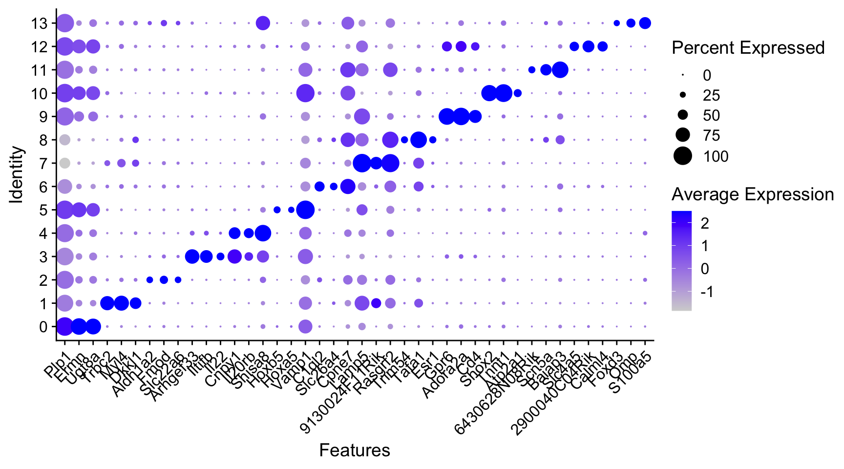
Now, we can check whether the expression pattern corresponds with the cluster, e.g. the top marker of cluster 3:
SpatialDimPlot(seu,
               cells.highlight = CellsByIdentities(object = seu,
                                                   idents = 7)) +
  plot_layout(guides='collect') &
theme(legend.position = "none") 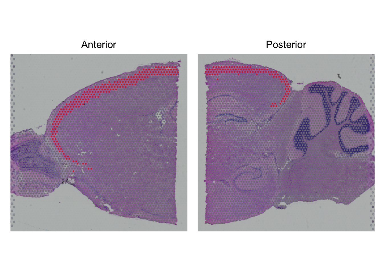
SpatialPlot(seu,
            features = top_markers$gene[top_markers$cluster == 7][1],
pt.size.factor = 2) 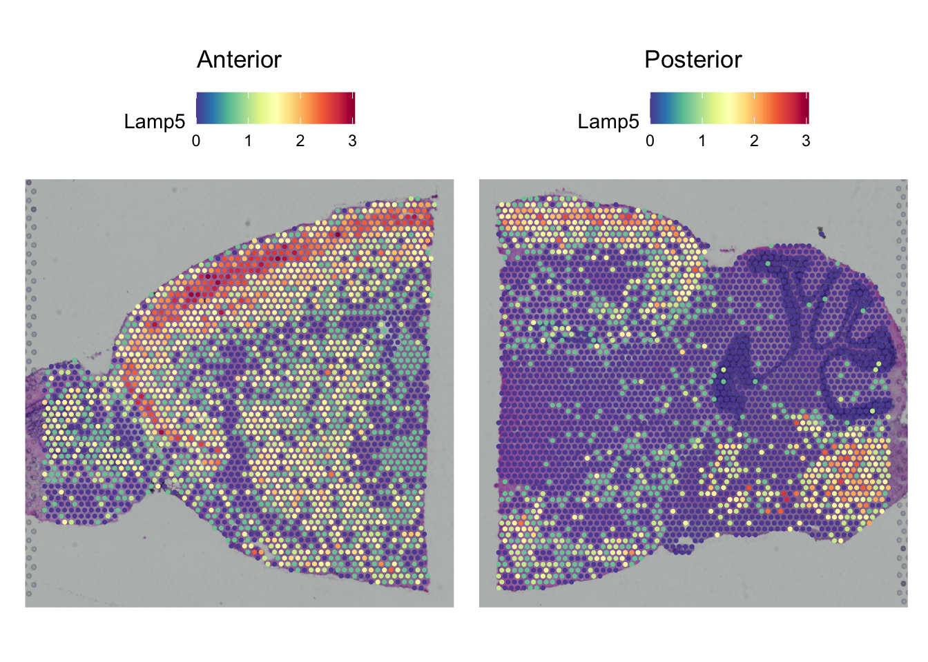
ImportantExercise
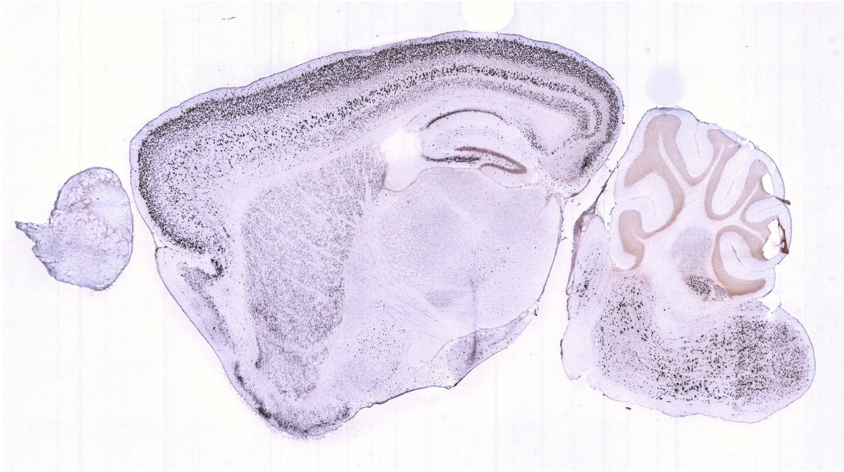
What kind of tissue is cluster 7 you think? Does the mouse brain atlas show similar patterns for this gene?
Compare the expression to the images at Allen Brain Atlas to figure out the tissue type.
To compare the expression, go to mouse.brain-map.org, type the gene name in the search box. Select the gene entry in the sagittal plane, click ‘View selections’ at the left bottom of the page. Select a similar slice (i.e. in the middle of the brain).
TipAnswer
Based on the comparison of the brain atlas it seems to be layer 2/3 of the isocortex.
It has similar expression based on in-situ hybridization from the brain atlas. Also expression in the striatium and medulla correspond.
ImportantExercise
Create the same visualization for cluster 0. What is the top marker? Can you guess what kind of cells this tissue is mostly comprised of?
The marker is expressed in many spots, and therefore it is not part of specific cell groups. Therefore, check out the gene at e.g. wikipedia.
TipAnswer
SpatialDimPlot(seu,
               cells.highlight = CellsByIdentities(object = seu,
                                                   idents = 0)) +
  plot_layout(guides='collect') &
theme(legend.position = "none") 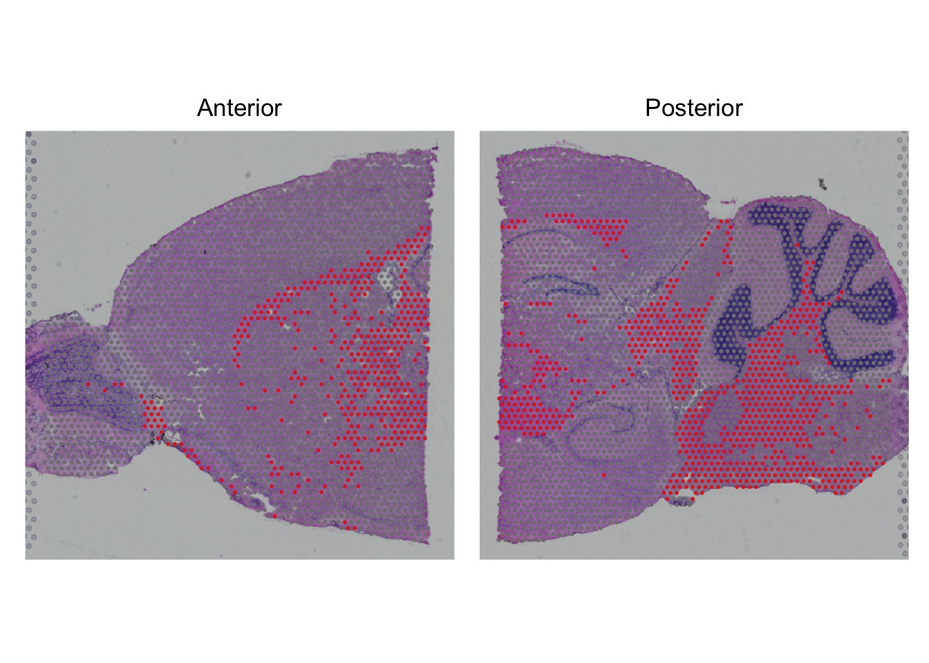
SpatialPlot(seu,
            features = top_markers$gene[top_markers$cluster == 0][1],
pt.size.factor = 2) 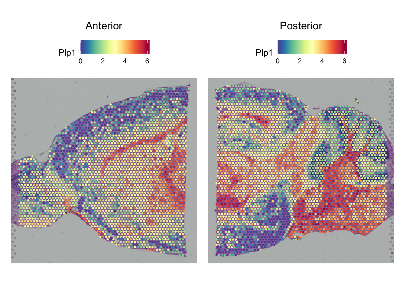
The top gene is Plp1 which protein is an important component of the myelin sheets of neurons. Therefore cluster 0 seems to represent the white matter of the brain.
Bonus exercise: spatially variable features
In stead of looking for features that are variable among all spots, you can also identify that mainly vary in space, i.e. while taking spot distance into account:
# take the output of part 3 (non-integrated and non-clustered)
seu_list <- readRDS("output/seu_part3.rds")

# we only do Anterior for now
DefaultAssay(seu_list$Anterior) <- "SCT"

seu_list$Anterior <-
  FindSpatiallyVariableFeatures(
    seu_list$Anterior,
    selection.method = "moransi",
    features = VariableFeatures(seu_list$Anterior)
  )

spatialFeatures <-
  SVFInfo(seu_list$Anterior, method = "moransi", status = TRUE)

spatialFeatures <-
  spatialFeatures |> arrange(rank)
ImportantExercise
Run the code and plot the top spatial variable genes.
The spatial features are ordered already ordered, so you can get them with e.g.
rownames(spatialFeatures)[1:4]Any interesting marker genes in there?
TipAnswer
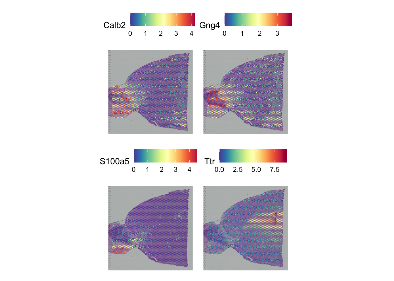
SpatialPlot(seu_list$Anterior,
            features = rownames(spatialFeatures)[1:4],
            ncol = 2)