Setup

Login and set up

If you are enrolled in the course, log on the server with the provided link, username, and password. The environment on the server contains all the necessary software pre-installed.

Create a project

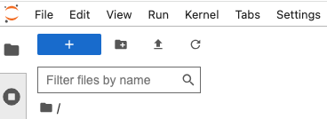
Now that you have access to an environment with the required installations, we will set up a project in a new directory. On the top right choose the “+” button.

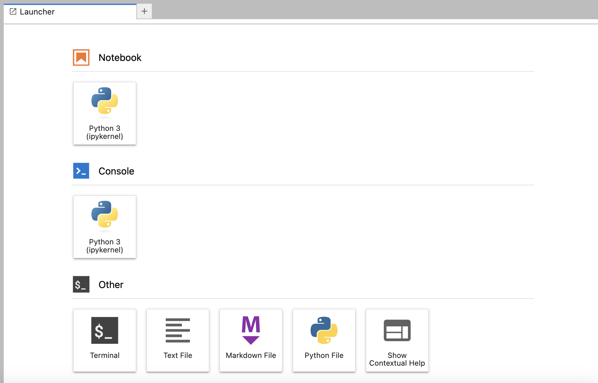
A new tab will open that allows you to choose between many options. The two most important ones are: 1. Other => Terminal 2. “Notebook => Python 3 (ipykernel)

Option (1) opens a command line prompt, which will be necessary for downloading the data and running cellranger. For the other exercises in Python, you will write your code in a Jupyter Lab notebook, which can be opened with the option (2). A Jupyter notebook is like a virtual laboratory notebook: you enter code into different “cells” and run those lines of code to read/write data, perform analyses, and make data visualizations. Also, a Jupyter notebook can be re-run multiple times to produce the same (reproducible) output!

When you open the terminal window, it will look like this:

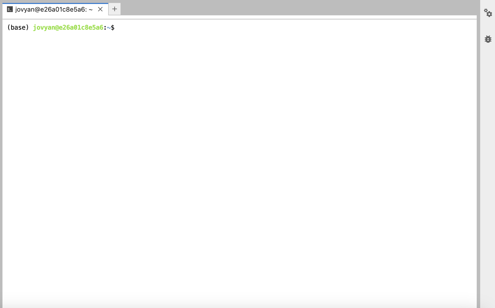
At the top are the various tabs corresponding to your different terminal and jupyter notebooks that are currently open.

If you instead open a Jupyter notebook (under Notebook > Python 3 (ipykernel)), it will look like this:

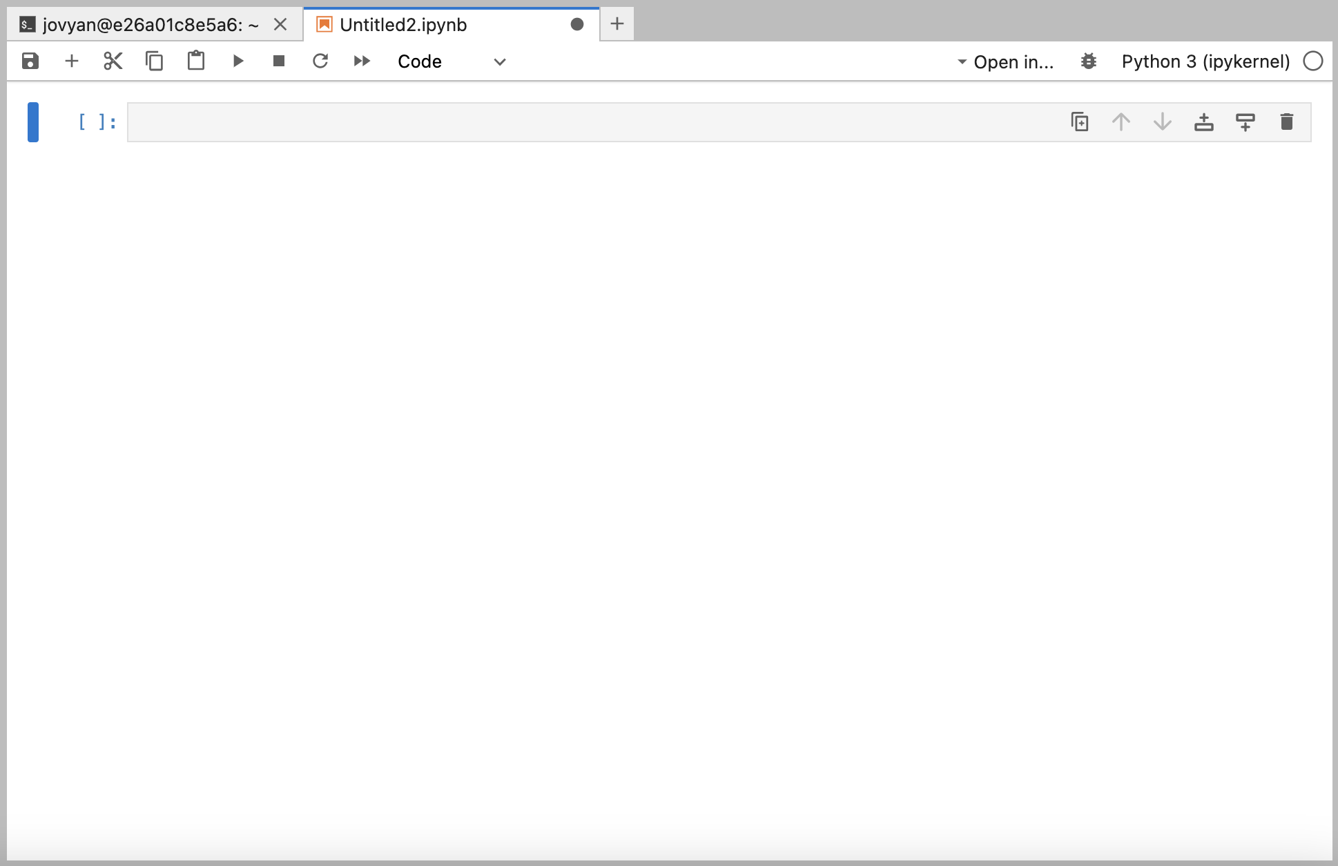
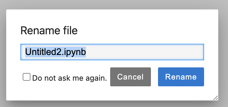
To rename a Jupyter notebook, type command+S (ctrl+S on a PC) and enter a name relevant to the analysis you will be performing in that specific notebook.

At the top of the Jupyter notebook, there are various buttons that allow you to interact with the notebook.

From left to right: - “SAVE” button (saves the notebook) - “ADD new code cell” button (adds a new cell where you can write code) - “CUT currently selected code cell” - “COPY currently selected code cell” - “RUN currently selected code cell” - “STOP running currently selected code cell” - “RESTART notebook” - “RUN ALL code cells in notebook”

You can also run a selected code cell by clicking on it and entering SHIFT + RETURN (SHIFT + ENTER on a PC).

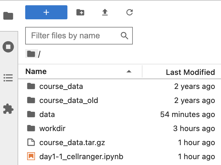
On the left hand side of the page, you will see your current directory containing various notebooks, data files, and folders that you create throughout the course. For example:

Downloading the course data

To download and extract the dataset, copy-paste these commands inside the terminal tab:

wget https://single-cell-transcriptomics-python.s3.eu-central-1.amazonaws.com/course_data.tar.gz
tar -xvf course_data.tar.gz
rm course_data.tar.gz

If on Windows

If you’re using Windows, you can directly open the link in your browser, and downloading will start automatically. Unpack the tar.gz file in the directory where you want to work in during the course.

Have a look at the data directory you have downloaded. It should contain the following:

course_data
├── count_matrices
│   ├── ETV6-RUNX1_1
│   │   └── outs
│   │       └── filtered_feature_bc_matrix
│   │           ├── barcodes.tsv.gz
│   │           ├── features.tsv.gz
│   │           └── matrix.mtx.gz
│   ├── ETV6-RUNX1_2
│   │   └── outs
│   │       └── filtered_feature_bc_matrix
│   │           ├── barcodes.tsv.gz
│   │           ├── features.tsv.gz
│   │           └── matrix.mtx.gz
│   ├── ETV6-RUNX1_3
│   │   └── outs
│   │       └── filtered_feature_bc_matrix
│   │           ├── barcodes.tsv.gz
│   │           ├── features.tsv.gz
│   │           └── matrix.mtx.gz
│   ├── PBMMC_1
│   │   └── outs
│   │       └── filtered_feature_bc_matrix
│   │           ├── barcodes.tsv.gz
│   │           ├── features.tsv.gz
│   │           └── matrix.mtx.gz
│   ├── PBMMC_2
│   │   └── outs
│   │       └── filtered_feature_bc_matrix
│   │           ├── barcodes.tsv.gz
│   │           ├── features.tsv.gz
│   │           └── matrix.mtx.gz
│   └── PBMMC_3
│       └── outs
│           └── filtered_feature_bc_matrix
│               ├── barcodes.tsv.gz
│               ├── features.tsv.gz
│               └── matrix.mtx.gz
└── reads
    ├── ETV6-RUNX1_1_S1_L001_I1_001.fastq.gz
    ├── ETV6-RUNX1_1_S1_L001_R1_001.fastq.gz
    └── ETV6-RUNX1_1_S1_L001_R2_001.fastq.gz

20 directories, 21 files

This data comes from:

Caron M, St-Onge P, Sontag T, Wang YC, Richer C, Ragoussis I, et al. Single-cell analysis of childhood leukemia reveals a link between developmental states and ribosomal protein expression as a source of intra-individual heterogeneity. Scientific Reports. 2020;10:1–12. Available from: http://dx.doi.org/10.1038/s41598-020-64929-x

We will use the reads to showcase the use of cellranger count. The directory contains only reads from chromosome 21 and 22 of one sample (ETV6-RUNX1_1). The count matrices are output of cellranger count, and we will use those for the other exercises in R.