import scanpy as sc
import pandas as pd # for handling data frames (i.e. data tables)
import numpy as np # for handling numbers, arrays, and matrices
import matplotlib.pyplot as plt # plotting package
import seaborn as sns # plotting packageData Integration
Download Presentation: Dimensionality Reduction and Integration
Exercise 0: Before we continue in this notebook with the next steps of the analysis, we need to load our results from the previous notebook using the sc.read_h5ad function and assign them to the variable name adata. Give it a try!
For simple integration tasks, it is worth first trying the algorithm Harmony. The harmonypy package is a port of the original tool in R. Harmony uses a variant of singular value decomposition (SVD) to embed the data, then look for mutual nearest neighborhoods of similar cells across batches in the embedding, which it then uses to correct the batch effect in a locally adaptive (non-linear) manner.
import harmonypy as hmExercise 1: Harmonypy operates on the principal components you previous obtained using the command sc.tl.pca. These are stored in your adata object under the .obsm field as X_pca. Can you extract these and store them in a variable named mat_PC in order to provide them directly to harmonypy in the following code cell?
adata = sc.read_h5ad("PBMC_analysis_SIB_tutorial3.h5ad")
mat_PC = adata.obsm["X_pca"]
Exercise 2: Next, we run harmony on the data to correct for any batch effects. We must specify with vars_use the metadata column name in adata.obs that we would like to correct for. Use the SHIFT+TAB option in Jupyter notebook to read about the harmony function’s required arguments, and run the command!
We can then visualize the extent to which each of the principal components was rescaled by harmonypy to correct for batch effects.
pc_std = np.std(ho.Z_corr, axis=1).tolist()sns.scatterplot(x=range(0, len(pc_std)), y=sorted(pc_std, reverse=True))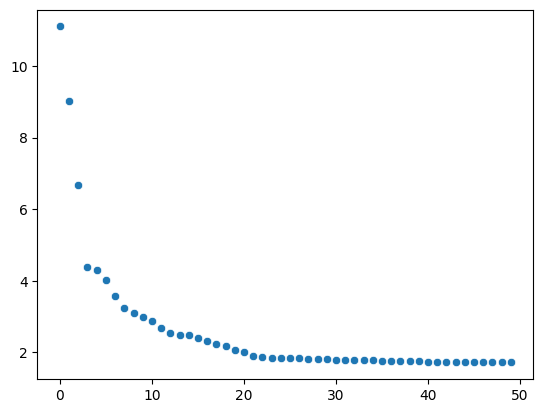
Finally, we store the results in our adata as X_pcahm variable.
adata.obsm["X_pcahm"] = ho.Z_corr.transpose()Exercise 3: Now that we have used harmony to correct for batch effects in our principal components, we want to rerun the sc.pp.neighbors and sc.tl.umap steps from our previous exercises, to obtain a new UMAP representation. Write those commands out below to obtain your new UMAP. Important: when running sc.pp.neighbors, you must specify that you would like to use the harmony-adjusted PCs and not the original, unadjusted ones. To do this, specify the optional argument use_rep=X_pcahm!
Exercise 4: Finally, visualize your UMAP with sc.pl.umap. How does the embedding compare to the one obtained prior to running harmony?
sc.pl.umap(adata, color=["sample"])/home/alex/anaconda3/envs/sctp/lib/python3.8/site-packages/scanpy/plotting/_tools/scatterplots.py:394: UserWarning: No data for colormapping provided via 'c'. Parameters 'cmap' will be ignored
cax = scatter(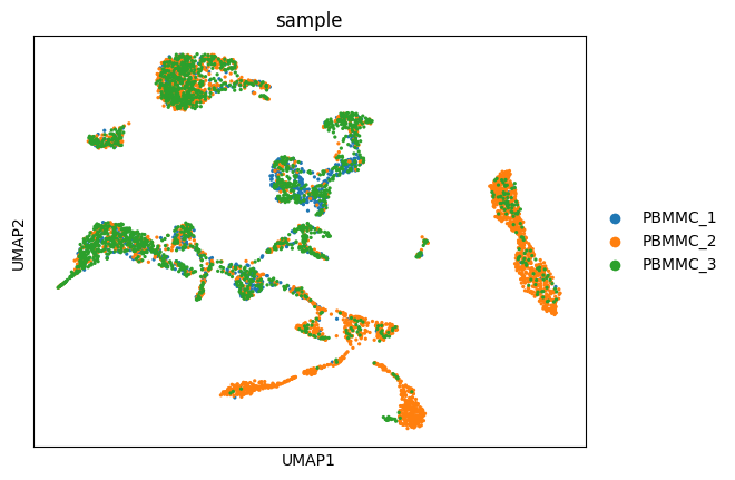
adata.write_h5ad("PBMC_analysis_SIB_tutorial4.h5ad") # save your results!