Exercise 3

ChIP and RNA sequencing data plots

Learning Objectives

By the end of this exercise, you will be able to:

• Load and explore SummarizedExperiment objects for ChIP-seq and RNA-seq data.
• Visualize ChIP-seq signal enrichment across genomic regions using the EnrichedHeatmap package.
• Generate and interpret RNA-seq expression heatmaps using the ComplexHeatmap package.
• Transform RNA-seq data to highlight differential expression using log fold-change.
• Annotate heatmaps with sample metadata to enhance interpretability.
• Split and visualize RNA-seq data based on gene regulation status (up- or down-regulated).
• Compare and reflect on the similarities and differences in visualization techniques between ChIP-seq and RNA-seq data.

Load Libraries

library(SummarizedExperiment)
library(EnrichedHeatmap)
library(gUtils)
library(rtracklayer)
library(circlize)

ChIP-seq SE object

Here we load the SummarizedExperiment for the ChIP-seq data

h3k4me3 <- readRDS("data/h3k4me3_se.rds")
h3k4me1 <- readRDS("data/h3k4me1_se.rds")
h3k27me3 <- readRDS("data/h3k27me3_se.rds")
h3k27ac <- readRDS("data/h3k27ac_se.rds")

Question 1

Similar to ATAC-seq data, please create EnrichedHeatmap for all ChIP-seq datasets and observe difference in genome activity at different genomic regions.

RNA-seq data

rna <- readRDS("data/rna_se.rds")

Heatmap of counts

For RNA-seq data, we use ComplexHeatmap package to make heatmaps

Heatmap(matrix = assay(rna, "logCPM"), 
        name = "RNA", 
        cluster_columns = FALSE, 
        show_row_names = FALSE
)

Warning: The input is a data frame-like object, convert it to a matrix.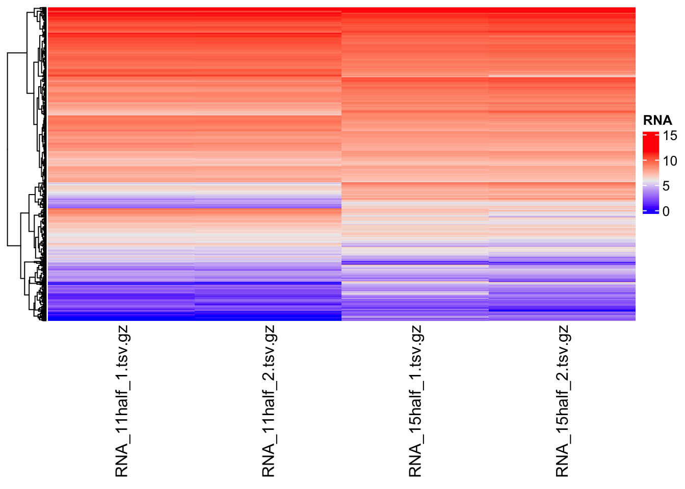

Changing visualization to fold change

counts <- assay(rna, "logCPM") - rowMeans(
  assay(rna, "logCPM")[, grep(pattern = "11half", x = colnames(assay(rna, "logCPM")),
                              value = T)]
)

Heatmap(matrix = counts, 
        name = "RNA", 
        cluster_columns = FALSE, 
        show_row_names = FALSE
)

Warning: The input is a data frame-like object, convert it to a matrix.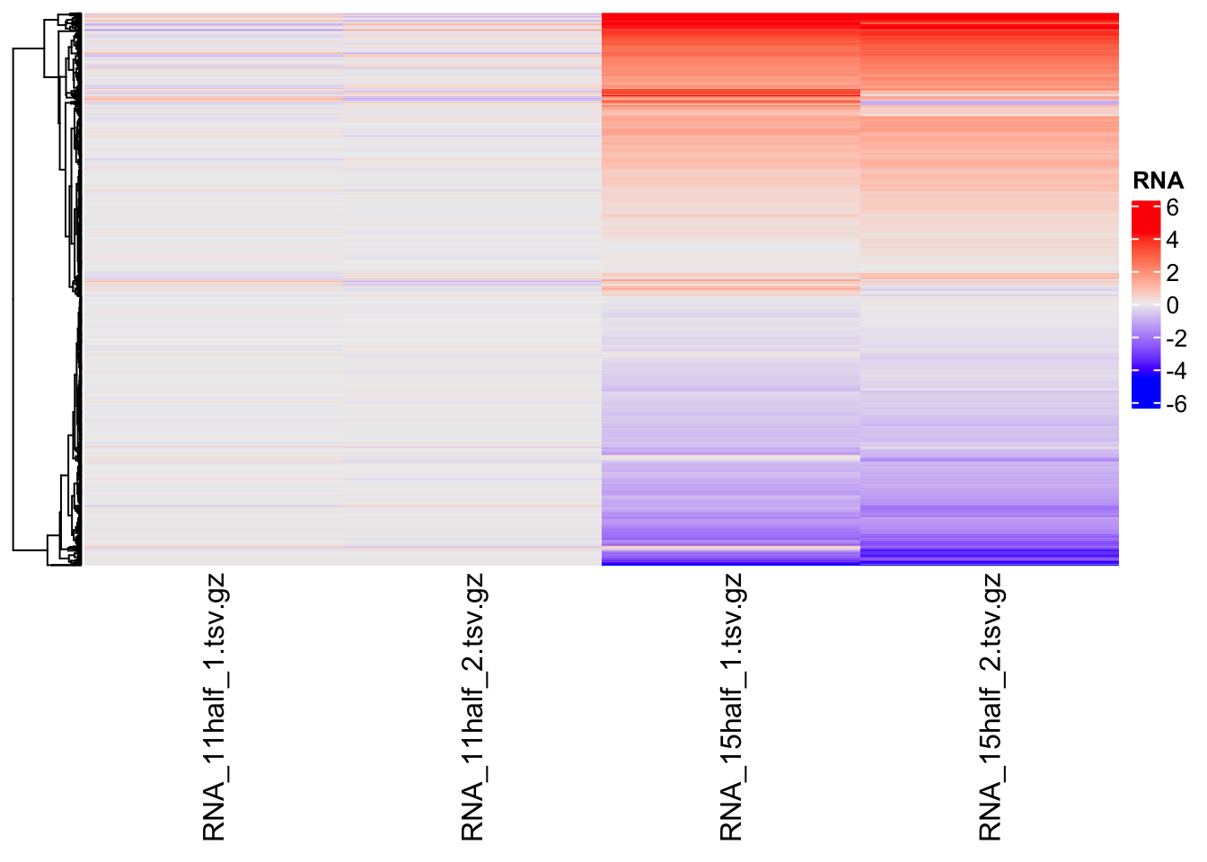

It is now more clear, which genes are up-regulated and which are down-regulated.

Adding colum annotations

colData(rna)

DataFrame with 4 rows and 2 columns
                                 sample    group
                            <character> <factor>
RNA_11half_1.tsv.gz RNA_11half_1.tsv.gz   11half
RNA_11half_2.tsv.gz RNA_11half_2.tsv.gz   11half
RNA_15half_1.tsv.gz RNA_15half_1.tsv.gz   15half
RNA_15half_2.tsv.gz RNA_15half_2.tsv.gz   15half

We can add groups information to the heatmap

Heatmap(matrix = counts, 
        name = "RNA", 
        cluster_columns = FALSE, 
        show_row_names = FALSE, 
        show_column_names = FALSE,
        top_annotation = HeatmapAnnotation(df = colData(rna)[,2,drop = FALSE]),
        width = unit(4, "cm"),
        height = unit(8, "cm"),
        heatmap_legend_param = list(
            at = scales::pretty_breaks(n = 3)(range(counts, na.rm = TRUE)), 
            title = "RNA"
        )
)

Warning: The input is a data frame-like object, convert it to a matrix.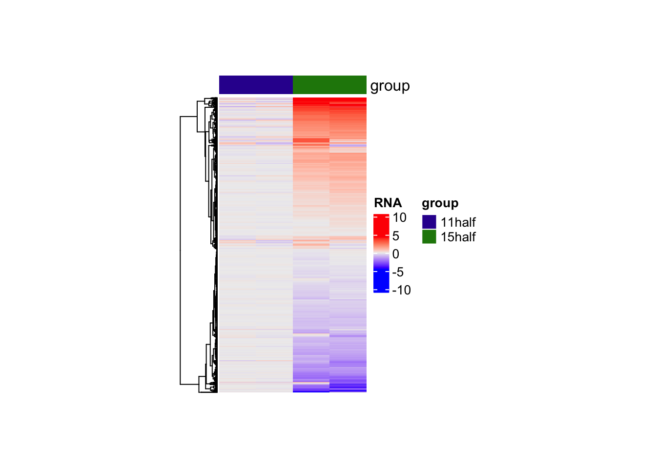

Question 2

Similar to EnrichedHeatmap, we can also split RNA-seq data based on logFC. Can you try to do this?

Tip

logFC <- rowData(rna)[,"logFC"]
names(logFC) <- rownames(rowData(rna))

logFC <- ifelse(logFC > 0, "Up regulated", "Down regulated")

Heatmap(matrix = counts, 
        name = "RNA", 
        cluster_columns = FALSE, 
        show_row_names = FALSE, 
        show_column_names = FALSE,
        top_annotation = HeatmapAnnotation(df = colData(rna)[,2,drop = FALSE]),
        width = unit(4, "cm"),
        height = unit(8, "cm"),
        heatmap_legend_param = list(
            at = scales::pretty_breaks(n = 3)(range(counts, na.rm = TRUE)), 
            title = "RNA"
        ),
        row_split = logFC
)

Warning: The input is a data frame-like object, convert it to a matrix.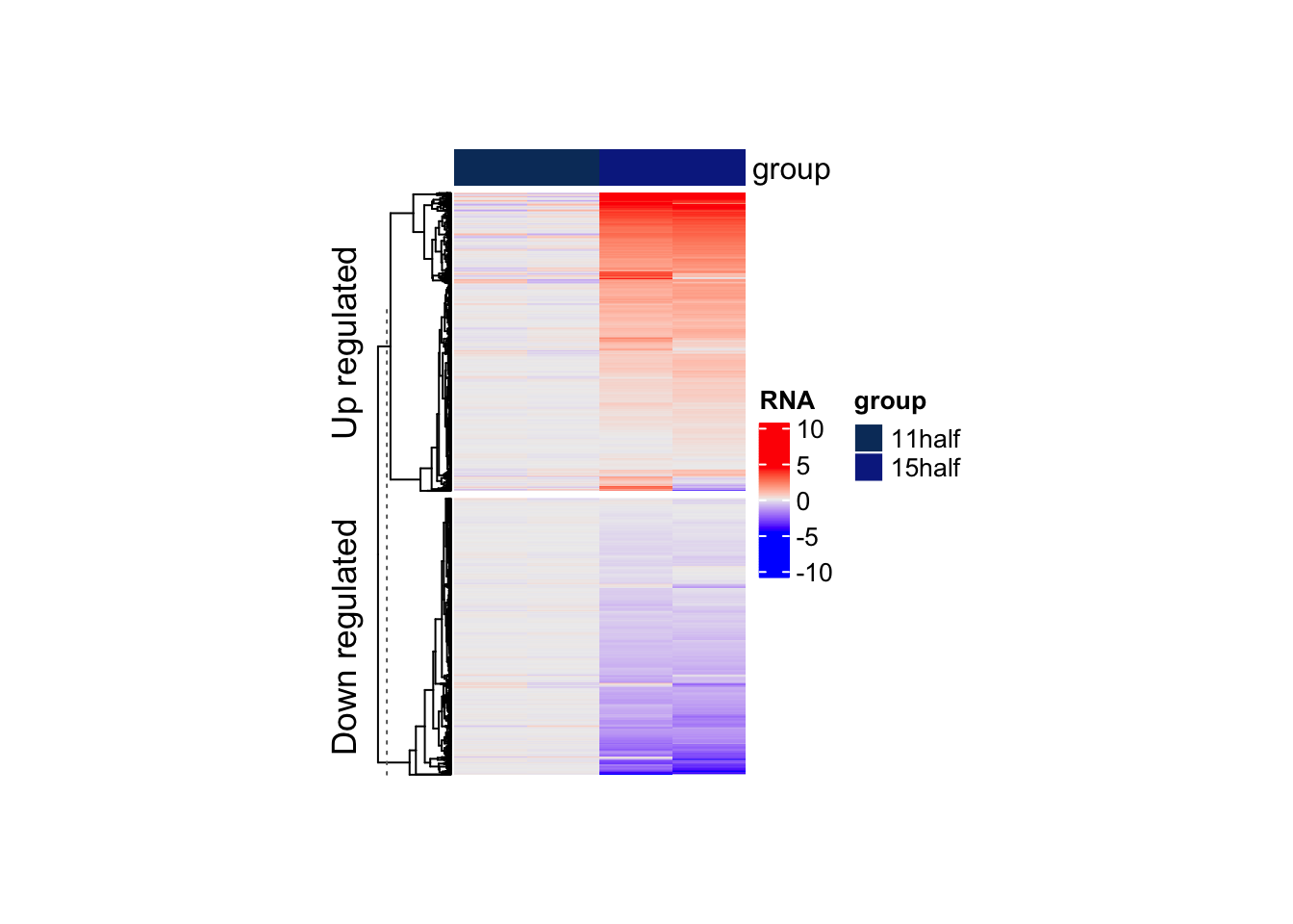

Important

Heatmap and EnrichedHeatmap have a lot of options in common.