Exercise 1B: SpatialFeatureExperiment - Xenium

Learning Objectives

By the end of this exercise, you will be able to:

• Understand the structure of a SpatialFeatureExperiment object.
• Explain when SpatialFeatureExperiment is useful compared with SpatialExperiment.
• Access cell-level metadata and spatial coordinates from Xenium data.
• Inspect geometry information such as cell or nucleus boundaries.
• Compare the Xenium representation with the Visium HD representation from Exercise 1A.

Libraries

library(SpatialFeatureExperiment)
library(SpatialExperiment)
library(Voyager)
library(ggplot2)
library(patchwork)
library(scuttle)
library(sfarrow)
library(HDF5Array)

Input data

Next, will work with the 10X Xenium dataset from the P2 sample (human colorectal cancer study by Oliveira et al).

This slide is a serial section of the sample used in Exercise 1A, so the two datasets are biologically related but not the exact same physical tissue section.

Imaging-based spatial transcriptomics platforms detect a targeted panel of a few hundred to a few thousand genes in situ at subcellular resolution, decoding each transcript over multiple rounds of imaging and assigning it to a segmented cell.

The full Xenium output is very large and includes cell boundaries, nucleus boundaries, transcript locations, morphology images, and expression matrices. For this exercise, for practical reasons we use a region of interest, selected to approximately match the region of interest used in Exercise 1A, and only include some of the layers in the imported compact course folder. This makes the two exercises comparable while avoiding a full image-registration workflow during the practical (but see this section from the OSTA book for some info on this process)

# Define the region of interest
roi_xenium <- c(
  xmin = 2200,
  xmax = 4500,
  ymin = 2500,
  ymax = 4900
)
roi_xenium

xmin xmax ymin ymax 
2200 4500 2500 4900 

We import the Xenium output with flip = "none" so the exercise uses the native Xenium coordinate orientation. We will see below that this differs from the coordinate system used by the Visium HD platform, which can be accounted for at the import stage, or later for when visualizing the data, which is what we chose to do for this practical. We import the compact Xenium output into a SpatialFeatureExperiment object:

# Import data into a SpatialFeatureExperiment object
sfe_full <- readXenium("data/Human_Colon_Cancer_P2/xenium/outs", flip = "none")

# Use unique Symbol for rownames
rownames(sfe_full) <- uniquifyFeatureNames(
  ID = rowData(sfe_full)$ID,
  names = rowData(sfe_full)$Symbol
)

dim(sfe_full)

[1]    541 340837

range(spatialCoords(sfe_full)[, 1])

[1]   20.43621 6654.75537

range(spatialCoords(sfe_full)[, 2])

[1]   19.4094 7269.5786

Then we subset it to the region of interest:

sfe <- sfe_full[, spatialCoords(sfe_full)[, 1] >= roi_xenium[["xmin"]] &
  spatialCoords(sfe_full)[, 1] <= roi_xenium[["xmax"]] &
  spatialCoords(sfe_full)[, 2] >= roi_xenium[["ymin"]] &
  spatialCoords(sfe_full)[, 2] <= roi_xenium[["ymax"]]]
rm(sfe_full)
sfe

class: SpatialFeatureExperiment 
dim: 541 52569 
metadata(1): Samples
assays(1): counts
rownames(541): ABCC8 ACP5 ... UnassignedCodeword_0330
  UnassignedCodeword_0338
rowData names(3): ID Symbol Type
colnames(52569): ablhnkec-1 ablhpkkh-1 ... oikdmkkf-1 oikeebja-1
colData names(9): transcript_counts control_probe_counts ...
  nucleus_area sample_id
reducedDimNames(0):
mainExpName: NULL
altExpNames(0):
spatialCoords names(2) : x_centroid y_centroid
imgData names(0):

unit: micron
Geometries:
colGeometries: centroids (POINT), cellSeg (MULTIPOLYGON), nucSeg (MULTIPOLYGON) 

Graphs:
sample01: 

ImportantExercise 1

Why is an object of the SpatialFeatureExperiment class used to store Xenium data?

Which information could not be represented by a simple spot- or bin-level SpatialExperiment?

TipAnswer

Xenium is an image-based spatial transcriptomics technology. In addition to a count matrix and cell coordinates, it can provide cell boundaries, nucleus boundaries, transcript locations, and morphology images.

SpatialFeatureExperiment extends SpatialExperiment with geometry support, making it better suited to storing and manipulating these spatial shapes.

Exploring the object

SpatialFeatureExperiment extends SpatialExperiment, which extends SingleCellExperiment, so familiar accessors still apply:

dim(sfe)

[1]   541 52569

colData(sfe) |> head()

DataFrame with 6 rows and 9 columns
           transcript_counts control_probe_counts control_codeword_counts
                   <integer>            <integer>               <integer>
ablhnkec-1               116                    0                       0
ablhpkkh-1               120                    0                       0
ablicbjh-1                89                    0                       0
ablilfnl-1                81                    0                       0
ablineen-1               145                    0                       0
ablioegm-1                71                    0                       0
           unassigned_codeword_counts deprecated_codeword_counts total_counts
                            <integer>                  <integer>    <integer>
ablhnkec-1                          0                          0          116
ablhpkkh-1                          0                          0          120
ablicbjh-1                          0                          0           89
ablilfnl-1                          0                          0           81
ablineen-1                          0                          0          145
ablioegm-1                          0                          0           71
           cell_area nucleus_area   sample_id
           <numeric>    <numeric> <character>
ablhnkec-1   75.0045      26.3261    sample01
ablhpkkh-1   72.7467      19.6881    sample01
ablicbjh-1   58.7031      26.1003    sample01
ablilfnl-1  132.1723           NA    sample01
ablineen-1   73.2434      28.7194    sample01
ablioegm-1   44.0273      30.9772    sample01

rowData(sfe) |> head()

DataFrame with 6 rows and 3 columns
                     ID      Symbol            Type
            <character> <character>     <character>
ABCC8   ENSG00000006071       ABCC8 Gene Expression
ACP5    ENSG00000102575        ACP5 Gene Expression
ACTA2   ENSG00000107796       ACTA2 Gene Expression
ADH1C   ENSG00000248144       ADH1C Gene Expression
ADRA2A  ENSG00000150594      ADRA2A Gene Expression
AFAP1L2 ENSG00000169129     AFAP1L2 Gene Expression

spatialCoords(sfe) |> head()

           x_centroid y_centroid
ablhnkec-1   3422.334   2507.607
ablhpkkh-1   3416.419   2512.555
ablicbjh-1   3428.145   2502.129
ablilfnl-1   3437.918   2514.156
ablineen-1   3430.172   2518.024
ablioegm-1   3447.884   2615.741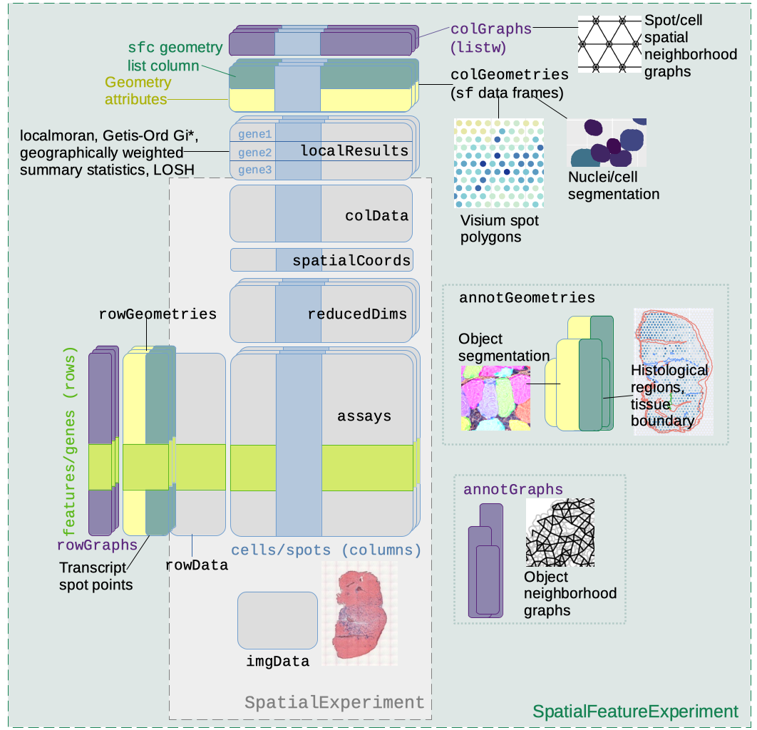

Overview of the SpatialFeatureExperiment class structure

Note: The practical Exercise 1C uses the segmented output of the Visium HD dataset used in Exercise 1A, which will also be stored into a SpatialFeatureExperiment object.

ImportantExercise 2

Check the dimensions and metadata of the sfe object.

Questions:

• What do the columns represent?
• What do the rows represent?
• What differs compared to the Visium HD spe object in Exercise 1A?
• What is stored in the main assay?

TipAnswer

In this object, columns represent segmented cells, while rows represent genes. This differs from the Visium HD slide stored in a SpatialExperiment object, where columns represent spatial bins rather than segmented cells.

ncol(sfe)

[1] 52569

nrow(sfe)

[1] 541

We notice that the number of features is small (541) as the Xenium technology measures a targeted panel rather than the whole transcriptome.

assay(sfe)

<541 x 52569> sparse DelayedMatrix object of type "integer":
                        ablhnkec-1 ablhpkkh-1 ablicbjh-1 ... oikdllpb-1
                  ABCC8          0          0          0   .          0
                   ACP5          0          0          1   .          0
                  ACTA2          1          0          0   .          0
                  ADH1C          0          0          0   .          0
                 ADRA2A          0          0          0   .          0
                    ...          .          .          .   .          .
UnassignedCodeword_0289          0          0          0   .          0
UnassignedCodeword_0292          0          0          0   .          0
UnassignedCodeword_0298          0          0          0   .          0
UnassignedCodeword_0330          0          0          0   .          0
UnassignedCodeword_0338          0          0          0   .          0
                        oikdmkkf-1 oikeebja-1
                  ABCC8          0          0
                   ACP5          0          0
                  ACTA2          0          0
                  ADH1C          0          0
                 ADRA2A          0          0
                    ...          .          .
UnassignedCodeword_0289          0          0
UnassignedCodeword_0292          0          0
UnassignedCodeword_0298          0          0
UnassignedCodeword_0330          0          0
UnassignedCodeword_0338          0          0

The count matrix indicates the number of observed molecules for each of the 541 genes in each cell. This matrix is analogous to a UMI counts matrix in the Visium HD dataset.

Inspecting geometries

In addition to the slots from the SpatialExperiment object, one of the key features of SpatialFeatureExperiment is that it can store geometries associated with cells or features.

colGeometries(sfe)

List of length 3
names(3): centroids cellSeg nucSeg

ImportantExercise 3

Inspect the available column geometries in the Xenium object. To which biological structures do they correspond to? In which class are stored these objects?

TipAnswer

The available geometries include cell centroids, cell boundaries, and nucleus boundaries. These are commonly available for imaging-based spatial transcriptomics technologies, but the exact names depend on the reader functions and packages used to import the data.

colGeometries(sfe)[["centroids"]]

Simple feature collection with 52569 features and 0 fields
Geometry type: POINT
Dimension:     XY
Bounding box:  xmin: 2200.037 ymin: 2500.096 xmax: 4499.985 ymax: 4899.936
CRS:           NA
First 10 features:
                    geometry
1  POINT (3422.334 2507.607)
2  POINT (3416.419 2512.555)
3  POINT (3428.145 2502.129)
4  POINT (3437.918 2514.156)
5  POINT (3430.172 2518.024)
6  POINT (3447.884 2615.741)
7  POINT (3458.518 2625.128)
8  POINT (3452.199 2632.097)
9  POINT (3453.355 2612.359)
10 POINT (3453.873 2623.217)

The geometries are stored using “Simple Features” objects, which allow to encode spatial data and can be easily manipulated with the sf package

Visualizing Xenium cells

We can start with a simple scatterplot of the cells in the selected region of interest:

xy <- as.data.frame(spatialCoords(sfe))
names(xy)[1:2] <- c("x", "y")

ggplot(xy, aes(x = x, y = y)) +
  geom_point(size = 0.08, alpha = 0.4) +
  coord_fixed() +
  theme_bw() +
  labs(x = "x", y = "y")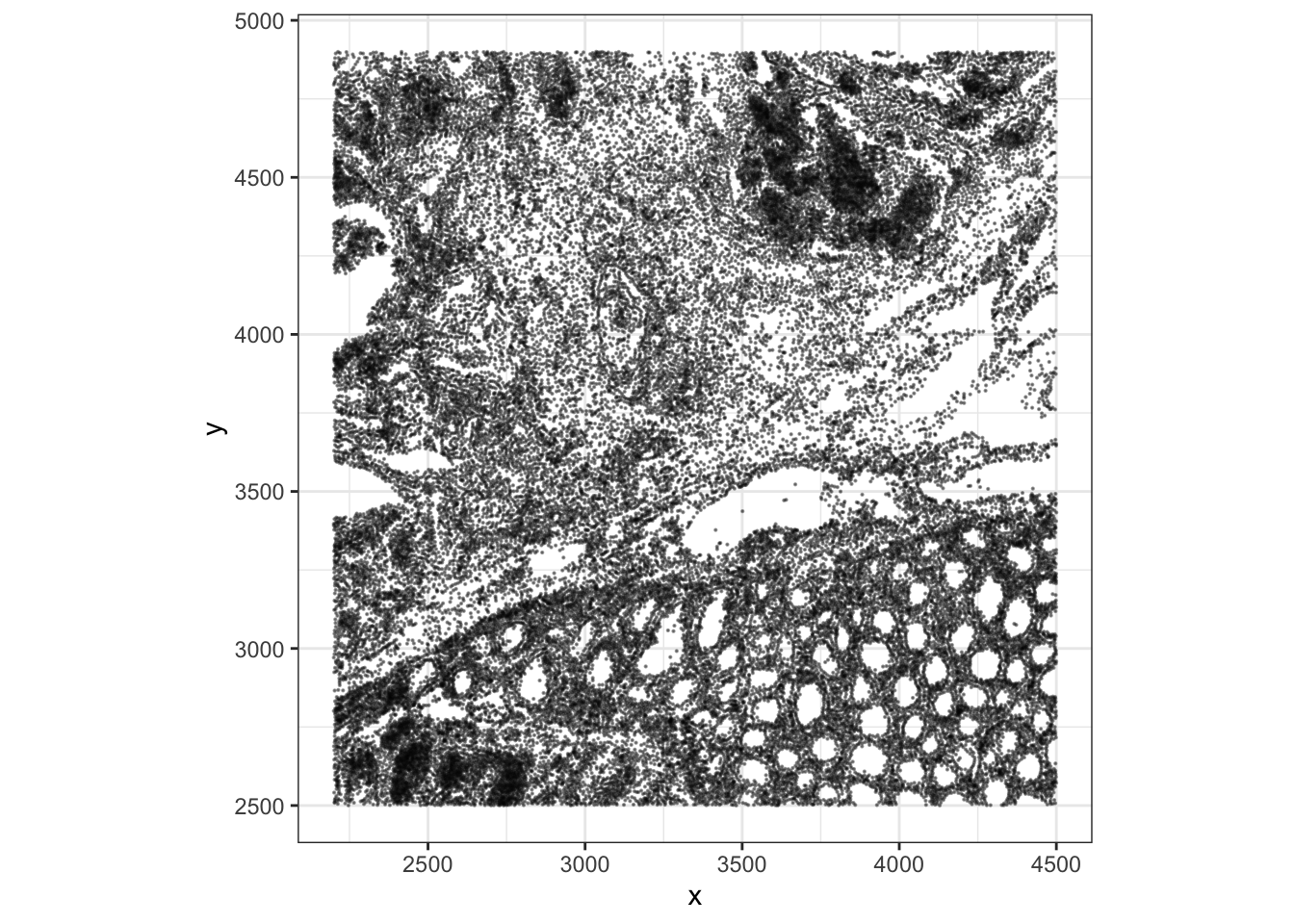

ImportantExercise 4

Compare this point-based visualization with the Visium HD plot from Exercise 1A. - What do you notice regarding the coordinates ? - What does one point represent in each dataset?

TipAnswer

The coordinate system differences between Visium HD and Xenium results in flipped image. It’s possible to simply correct this at the plotting step:

ggplot(xy, aes(x = -y, y = -x)) +
  geom_point(size = 0.08, alpha = 0.4) +
  coord_fixed() +
  theme_bw() +
  labs(x = "x", y = "y")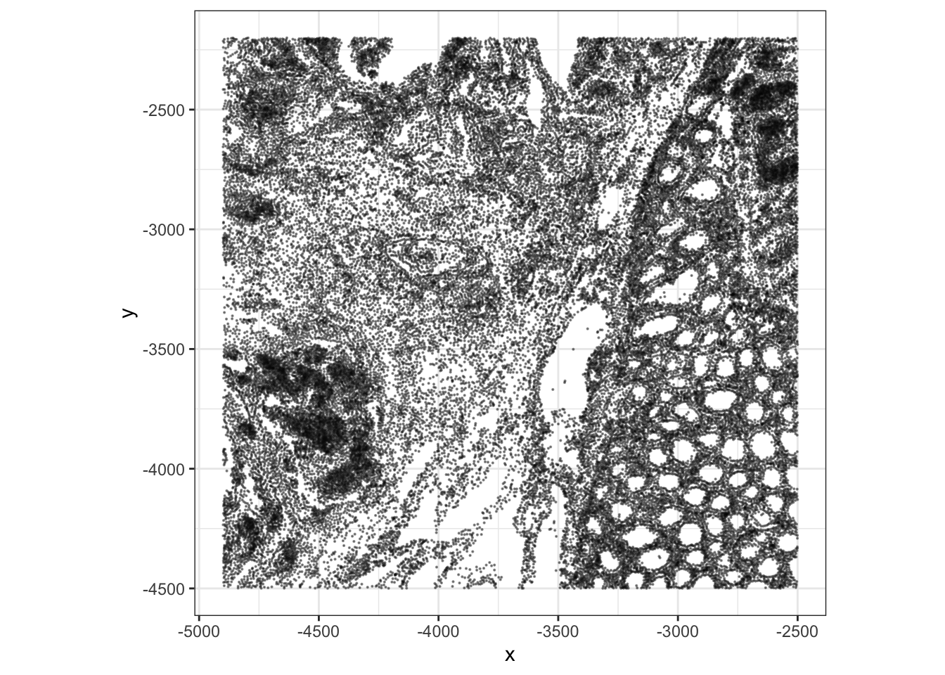

In the Visium HD exercise, each point or square represents a 16 um spatial bin. In the Xenium exercise, each point represents a segmented cell centroid. This is one of the key conceptual differences between binned sequencing-based spatial data and image-based cell-resolved spatial data.

We can also visualize expression for a marker gene. For example, PIGR is present in the Xenium panel and shows a clear spatial pattern in this region. We renamed the rows to gene symbols after import, which is why we can refer to this marker as "PIGR" rather than by its Ensembl ID. At this stage we plot the number of molecules since log-normalized counts will be introduced later in the course. The plotSpatialFeature() function from the Voyager package is handy:

plotSpatialFeature(sfe, "PIGR", exprs_values = "counts")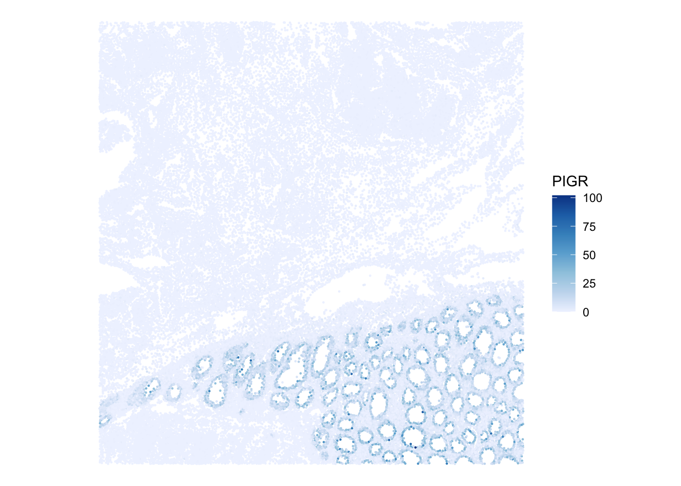

ImportantExercise 5

Choose another marker gene and visualize its spatial pattern.

How does the interpretation differ from plotting a gene on Visium HD bins? How does the expression of the same gene compares across platforms?

TipAnswer

The Xenium signal is measured over segmented cells, while the Visium HD binned signal aggregates molecules within fixed spatial bins. Xenium can therefore represent cell-level heterogeneity more directly, but it measures a targeted panel rather than the whole transcriptome.

Here is some code to plot the log of the molecule counts of the same gene across platforms in a comparable way:

xy <- data.frame(spatialCoords(sfe), colData(sfe), PIGR=counts(sfe)["PIGR",] + 1)
names(xy)[1:2] <- c("x", "y")
p_xen <- ggplot(xy, aes(x = -y, y = x, color=PIGR)) +
  geom_point(size = 0.2) +
  coord_fixed() +
  scale_color_gradient(trans = "log", low = "white", high = "red") +
  theme_bw() 

## load the object from Exercise 1A
spe <- loadHDF5SummarizedExperiment(dir="results/day1/", prefix="01.1a_spe_")
xy <- data.frame(spatialCoords(spe), colData(spe), PIGR=counts(spe)["PIGR",] + 1)
names(xy)[1:2] <- c("x", "y")
p_vis <- ggplot(xy, aes(x = x, y = y, color=PIGR)) +
  geom_point(size = 1, shape=15) +
  coord_fixed() +
  scale_color_gradient(trans = "log", low = "white", high = "red") +
  theme_bw() 

p_xen + p_vis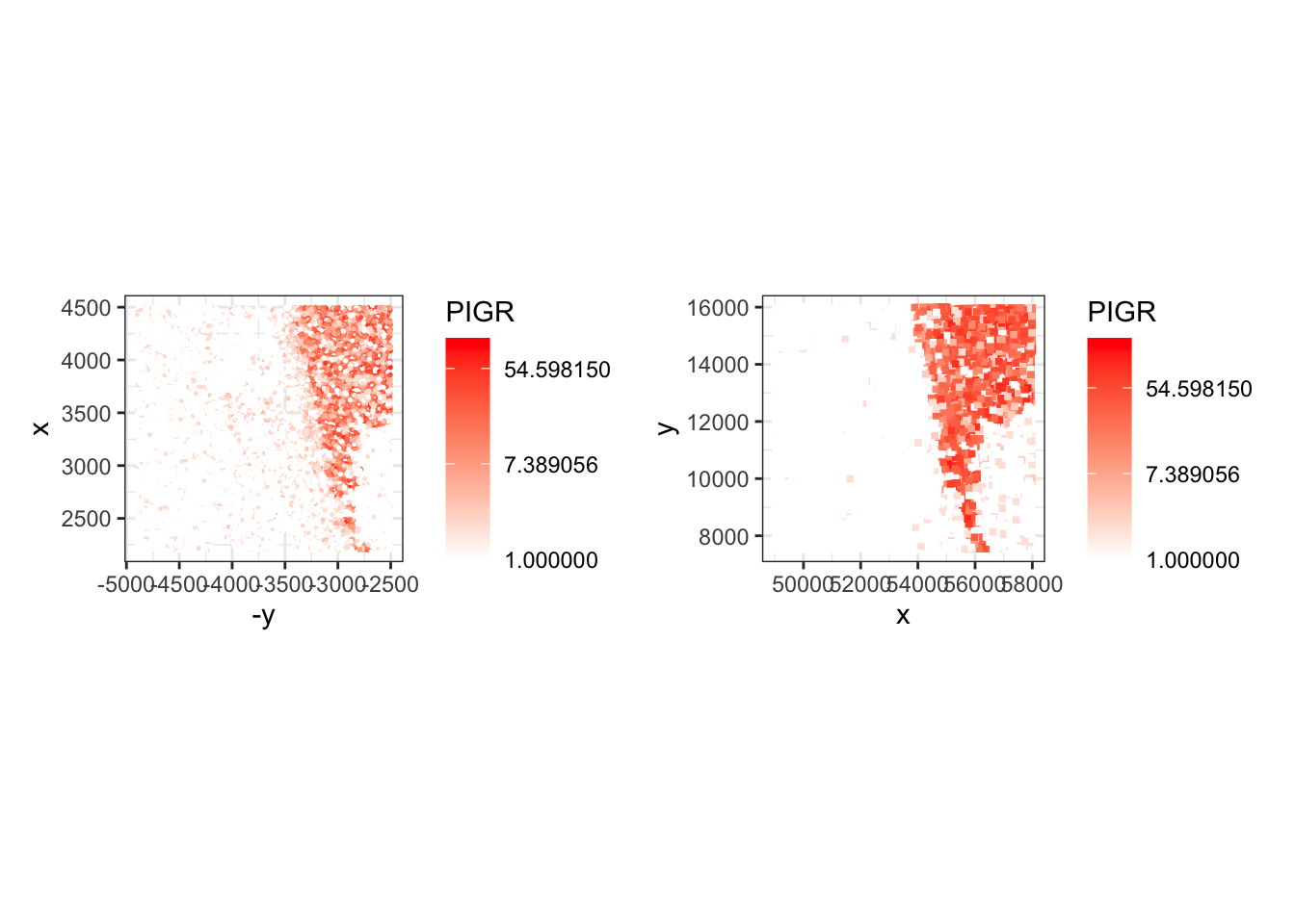

ImportantExercise 6

Use the plotSpatialFeature() function to visualize the cell segmentation mask, colored by cell area, and the nuclei segmentation mask, colored by nucleus area

TipAnswer

plotSpatialFeature(sfe, 
                   colGeometryName="cellSeg", 
                   features="cell_area")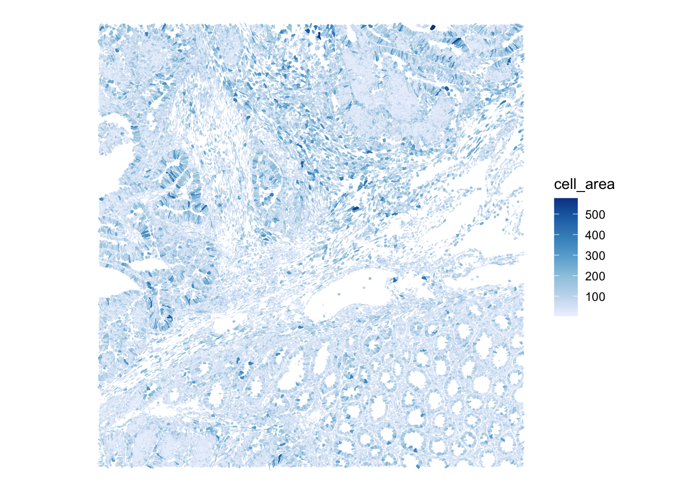 

plotSpatialFeature(sfe, 
                   colGeometryName="nucSeg", 
                   features="nucleus_area")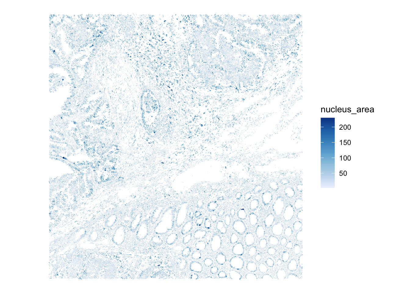 

Save the object

In the Exercise 1A we used the function saveHDF5SummarizedExperiment because the count matrix of the SpatialExperiment object is stored on-disk for efficiency.

As you could see above, the SpatialFeatureExperiment includes additional layers, and some of them are also not loaded in memory. This complicates things further and even saving the object with the saveHDF5SummarizedExperiment function does not allow to fully re-import it.

A nice way to save the object is to use the alabaster.sfe package, implementing a (language agnostic) format to represent SpatialFeatureExperiment on disk (see the ArtifactDB project). See the package vignette here.

dir.create("results/day1", showWarnings = FALSE, recursive = TRUE)

alabaster.sfe::saveObject(sfe, "results/day1/01.1b_sfe_xenium")

Clear your environment:

rm(list = ls())
gc()
.rs.restartR()

Important

Key Takeaways:

• SpatialFeatureExperiment is useful for geometry-rich spatial data.
• Xenium observations are cell-resolved, while the Visium HD object in Exercise 1A is bin-resolved.
• The P2 CRC subsets are designed to be comparable in course scope and approximate tissue region, not identical at cell level.