library(Banksy)
library(igraph)
library(ggspavis)
library(BayesSpace)
library(nnSVG)
library(HDF5Array) # For loading object
library(patchwork)
library(SpatialExperiment)
library(SpatialFeatureExperiment)
library(Voyager)
library(scran)
library(scater)
library(bluster)
library(SingleR)
library(qs2)
library(viridis)
library(RColorBrewer)
library(pheatmap)
library(alabaster.sfe)Exercise 6: Clustering and Domains
Clustering and Spatially-aware clustering
In the next section we will explore clustering methods for spatial transcriptomics data, including classical non-spatially aware and spatially-aware approaches.
Learning Objectives
By the end of this exercise, you will be able to:
- Perform non-spatially aware clustering using graph-based methods (Leiden clustering).
- Perform spatially-aware clustering using Bayesian modeling (BayesSpace) and graph-based methods (Banksy + Leiden).
- Visualize and compare clustering results from different methods on tissue slides.
Clustering
We will start by loading the normalized Visium HD dataset stored in the SpatialFeatureExperiment object generated in the previous exercise. It contains information on the HVGs and dimensionationality reduction computed with Banksy and PCA.
# Reload the SpatialFeatureExperiment object if not in the R session already
sfe <- readObject("results/day2/02.2_sfe/")
sfe
class: SpatialFeatureExperiment
dim: 18878 33763
metadata(2): resources spatialList
assays(2): counts logcounts
rownames(18878): OR4F5 SAMD11 ... DEPRECATED_ENSG00000291096
DEPRECATED_TRIM16L
rowData names(5): ID Symbol Type subsets_Mito hvg
colnames(33763): cellid_000080404-1 cellid_000080411-1 ...
cellid_000189331-1 cellid_000189341-1
colData names(31): sample_id area ... artifact sizeFactor
reducedDimNames(5): PCA_artifacts PCA PCA_banksy UMAP UMAP_banksy
mainExpName: Gene Expression
altExpNames(0):
spatialCoords names(2) : pxl_col_in_fullres pxl_row_in_fullres
imgData names(4): sample_id image_id data scaleFactor
unit:
Geometries:
colGeometries: centroids (POINT), cellSeg (POLYGON)
Graphs:
sample01: Non-spatial aware clustering
Clustering methods can be categorized into non-spatially aware, e.g., these include the methods classically used for scRNA-seq analysis, and spatially-aware methods. We will first explore non-spatially aware clustering using graph-based methods.
As commonly done in single-cell RNA-seq analysis, we can perform graph-based clustering using the Leiden algorithm on a shared nearest-neighbor (SNN) graph constructed from the PCA results.
# build cellular shared nearest-neighbor (SNN) graph
g <- makeSNNGraph(reducedDim(sfe, "PCA"), type="jaccard", k=20)
# cluster using Leiden community detection algorithm
k <- cluster_leiden(g, objective_function="modularity", resolution=0.6)
# assign cluster labels to sfe object
sfe$Leiden <- factor(k$membership)
table(sfe$Leiden)
   1    2    3    4    5    6    7    8    9
5515 4980 4141 3373 1375 4521 4321  784 4753
Spatialy aware clustering
Clustering methods can also incorporate spatial information to identify spatial domains or regions in the tissue.
Probabilistic: BayesSpace
The BayesSpace package performs spatially-aware clustering using a Bayesian modeling approach. Unfortunately it is not possible yet to use it on segmented data, see for example: https://github.com/edward130603/BayesSpace/issues/136
Exercise 1: Bonus
Go back to our binned data stored in a SpatialExperiment object to run BayesSpace. We need to quickly go through all the steps of normalization, HVG selection and dimensionality reduction.
spe <- loadHDF5SummarizedExperiment(dir="results/day1/", prefix="01.1a_spe_")
spe <- logNormCounts(spe)

dec <- modelGeneVarByPoisson(spe)
dec <- dec[order(dec$bio, decreasing = T), ]
hvg <- getTopHVGs(dec, n = 1000)
rowData(spe)$hvg <- rowData(spe)$Symbol %in% hvg

## non-spatial PCA
spe <- runPCA(spe, ncomponents = 10, subset_row = rowData(spe)$hvg)

# Banksy PCA (for comparison)
k <- 20   # consider first order neighbors
l <- 0.8 # use spatial information with weight lambda
a <- "logcounts" # assay to use
xy <- c("array_row", "array_col")  # spatial coordinate names
set.seed(123)
tmp <- computeBanksy(spe[rowData(spe)$hvg, ],
                     assay_name=a,
                     coord_names=xy,
                     k_geom=k,
                     parallel=T,
                     num_cores=4)
tmp <- runBanksyPCA(tmp,
                    lambda=l,
                    npcs=10)
reducedDim(spe, "PCA_banksy") <- reducedDim(tmp, "PCA_M0_lam0.8")


# Prepare data for 'BayesSpace'
# skipping PCA (already computed)
spe <- spatialPreprocess(spe, skip.PCA=TRUE)

# perform spatial clustering with 'BayesSpace'
# using 'd=10' PCs and targeting 'q=8' clusters
spe <- spatialCluster(spe, q=8, d=10, nrep=1e3, burn.in=100)
spe$BayesSpace <- factor(spe$spatial.cluster)
table(spe$BayesSpace)
   1    2    3    4    5    6    7    8
5343 3966 4931 3337  930 1916  773 1223
Graph-based: Banksy
We have computed spatially-aware principal components using Banksy already in the previous practical. We will now used these to perform SNN graph-based Leiden clustering, in order to obtain spatially-aware clusters. When building the SNN graph, we will use the same parameters we have used before for the non-spatially aware graph.
# perform SNN graph-based clustering on 'Banksy' PCs using
g <- buildSNNGraph(sfe, use.dimred="PCA_banksy", type="jaccard", k=20)
# cluster using Leiden community detection algorithm
k <- cluster_leiden(g, objective_function="modularity", resolution=0.2)
sfe$Banksy <- factor(k$membership)
table(sfe$Banksy)
   1    2    3    4    5    6
8708 9358 3463 1359 9888  987
Exercise 2: Bonus
Perform a similar graph-based clustering on Banksy PCs in the binned spe object
Comparison of results from the different clustering methods
Let’s visualize the clustering results from the different methods on the tissue slide.
## 2 methods to compare for the sfe object
ks <- c("Leiden", "Banksy")
plotSpatialFeature(sfe, features = ks)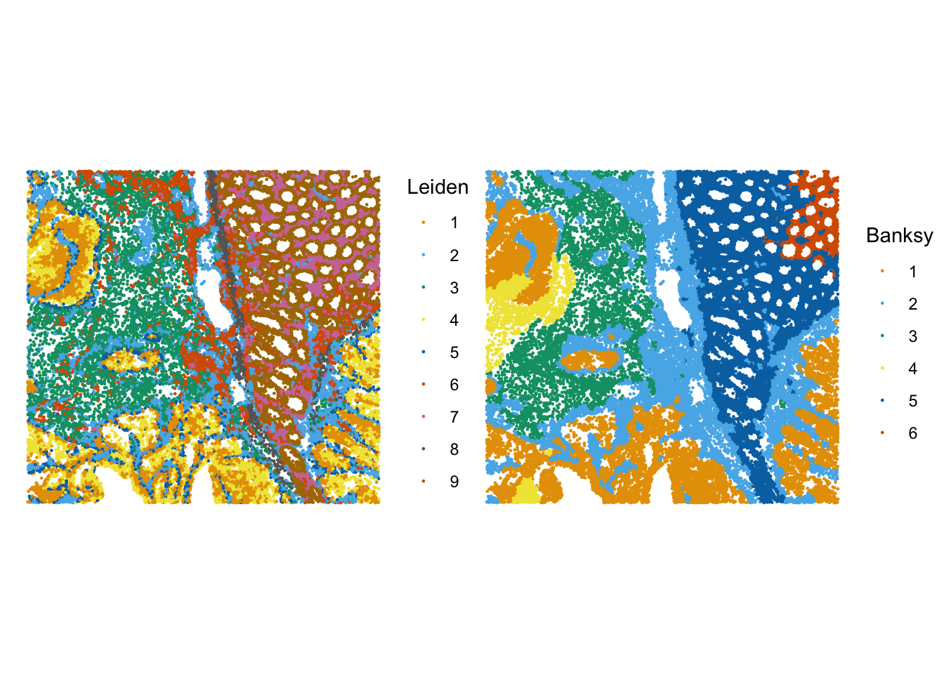
## If BayesSpace was run on the spe object
# Colorblind friendly palette
data("ditto_colors")
plotVisium(spe,
           annotate = "BayesSpace",
           zoom = TRUE,
           image = FALSE,
           point_size = 1.5,
           point_shape = 22) +
 scale_fill_manual(values = ditto_colors)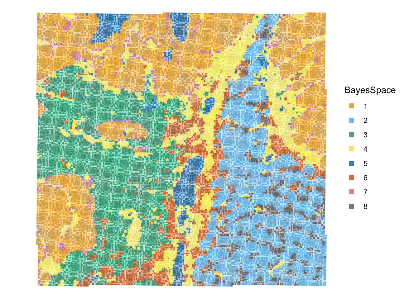
It can help us to visualise the clusters one by one, in order to better see their spatial distribution. We take as an example the Banksy clusters:
# plot selected clusters in order of frequency, highlighting cells assigned to cluster 'k'
lapply(names(sort(table(sfe$Banksy), decreasing = TRUE)), \(k) {
    sfe$foo <- sfe$Banksy == k
    sfe <- sfe[, order(sfe$foo)]
    plt <- plotSpatialFeature(sfe, features = "foo")
    plt + ggtitle(k) + guides(fill="none")
}) |>
  wrap_plots(nrow=2) &
  scale_color_manual(values=c("white", "red")) &
  theme(plot.title=element_text(hjust=0.5), legend.position="none")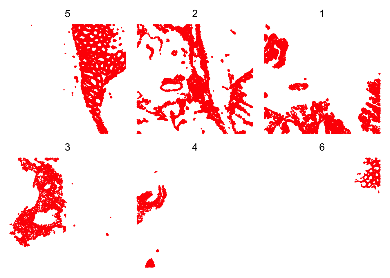
ImportantExercise 3
Visualise the clusters obtained with the 3 methods, and compare their spatial distribution. What do you observe?
What is the interpretation of a domain compared to a cluster?
Save the object
Save the SpatialFeatureExperiment object for the next steps:
alabaster.sfe::saveObject(sfe, "results/day2/02.3_sfe")Potentially save the SpatialExperiment object used in bonus exercises
saveHDF5SummarizedExperiment(spe,
  dir = "results/day2", prefix = "02.3_spe_", replace = TRUE,
  chunkdim = NULL, level = NULL, as.sparse = NA,
  verbose = NA
)
Clear your environment: