Exercise 4A: Visium HD Normalization

Normalization and scaling for Visium HD

In this exercise, we normalize the filtered Visium HD object from yesterday’s Exercise 2. Standard library-size normalization, as used for scRNA-seq analysis, is a useful starting point, but spatial data introduces additional challenges: total counts can vary because of local capture efficiency, tissue density, morphology, or real biology.

Learning objectives

By the end of this exercise, you will be able to:

Add log-normalized values to a Visium HD SpatialExperiment or SpatialFeatureExperiment object.
Inspect size factors and assay names.
Scale selected features for visualization and downstream multivariate methods.
Understand the principles of spatially-aware normalization and evaluate whether it could be useful for a given dataset.

Libraries

library(SpatialExperiment)
library(SpatialFeatureExperiment)
library(scuttle)
library(scrapper)
library(scater)
library(HDF5Array)
library(ggspavis)
library(alabaster.sfe)
library(Voyager)

Load the Visium HD object

We start with the filtered Visium HD object saved at the end of Exercise 2.

# Reload the SpatialFeatureExperiment object if not in the R session already
sfe <- readObject("results/day1/01.2_sfe_visium/")
sfe

class: SpatialFeatureExperiment 
dim: 18878 33763 
metadata(2): resources spatialList
assays(1): counts
rownames(18878): OR4F5 SAMD11 ... DEPRECATED_ENSG00000291096
  DEPRECATED_TRIM16L
rowData names(4): ID Symbol Type subsets_Mito
colnames(33763): cellid_000080404-1 cellid_000080411-1 ...
  cellid_000189331-1 cellid_000189341-1
colData names(30): sample_id area ... k90 artifact
reducedDimNames(1): PCA_artifacts
mainExpName: Gene Expression
altExpNames(0):
spatialCoords names(2) : pxl_col_in_fullres pxl_row_in_fullres
imgData names(4): sample_id image_id data scaleFactor

unit: 
Geometries:
colGeometries: centroids (POINT), cellSeg (POLYGON) 

Graphs:
sample01:

Log-normalization

The object contains raw counts. We use the scuttle::logNormCounts() function to compute size factors and add a logcounts assay.

Note

This function will deprecate soon and replaced by the faster scrapper::normalizeRnaCounts.se() function.

assayNames(sfe)

[1] "counts"

sfe <- logNormCounts(sfe)

Exercise 1

What assay was added to the Visium HD object? What do the size factors represent?

Answer

assayNames(sfe)

[1] "counts"    "logcounts"

summary(sizeFactors(sfe))

   Min. 1st Qu.  Median    Mean 3rd Qu.    Max. 
 0.1234  0.4716  0.7673  1.0000  1.2620  8.8843

The logcounts assay contains log-normalized expression values. The size factors adjust for differences in total count depth between cells.

Note

Other more advanced normalization methods exist for scRNA-seq data, which aim at adjusting for compositional biases across cells, for example scuttle::computePooledFactors(), or at stabilizing the variance of such low-counts data, for example Seurat:SCTranform()

We can inspect whether size factors have a spatial pattern.

colData(sfe)$sizeFactor <- sizeFactors(sfe)

plotSpatialFeature(
    sfe,
    colGeometryName = "cellSeg", features = "sizeFactor"
)

Exercise 2

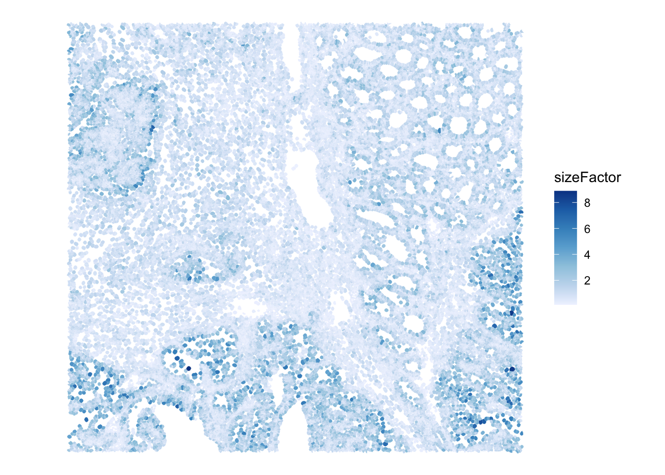
Do size factors show a spatial pattern across the tissue region? What biological or technical effects could explain this?

Scaling selected features

Normalization adjusts for differences in total counts between observations. Scaling is a different step: it centers and rescales features so that they can be compared on a common scale. This is often useful for multivariate methods such as PCA, clustering, or heatmaps, to avoid giving more weight to more highly expressed genes.

Here we demonstrate scaling on a small set of marker genes.

marker_genes <- c("PIGR", "CEACAM5", "MUC17", "OLFM4")
marker_genes <- intersect(marker_genes, rownames(sfe))
marker_genes

[1] "PIGR"    "CEACAM5" "MUC17"   "OLFM4"

scale_rows <- function(x) {
  t(base::scale(t(x)))
}

visium_scaled <- scale_rows(as.matrix(logcounts(sfe)[marker_genes, ]))
visium_scaled[, 1:5]

        cellid_000080404-1 cellid_000080411-1 cellid_000080412-1
PIGR            -0.4813121         -0.4813121         -0.4813121
CEACAM5          1.6156216         -0.8229917         -0.8229917
MUC17           -0.1642005         -0.1642005         -0.1642005
OLFM4           -0.3805620         -0.3805620         -0.3805620
        cellid_000080429-1 cellid_000080439-1
PIGR            -0.4813121         -0.4813121
CEACAM5          1.9094831          1.8186274
MUC17           -0.1642005         -0.1642005
OLFM4           -0.3805620         -0.3805620

Exercise 3

What does a positive scaled value mean for a gene in one cell? Why should scaling be applied after normalization rather than directly to raw counts?

Answer

A positive scaled value means that the cell has expression above the average for that gene, relative to the variation of that gene across the dataset. Scaling should be applied after normalization because raw counts are strongly affected by sequencing depth.

Optional: spatially-aware normalization

Optional discussion

In spatial transcriptomics, in addition to sequencing depth, total counts can vary because of tissue density, local capture efficiency, or morphological structures. Many of these factors are partially confounded with biology, for example with the differences observed across cell types.

Spatially-aware normalization methods try to account for spatial structure while avoiding the removal of true spatial biological signal. This is an active area of method development, cf. the OSTA book discussion about these issues. Packages such as SpaNorm can be explored as optional extensions, but their basic assumption might not apply to all tissues (e.g., the cell type composition is relatively homogenous in brain so spatial smoothing might be advantageous, but it is not in our colon sample, so is smoothing a good idea?)

For this course, we keep the required workflow simple and use logNormCounts(). When interpreting the downstream results, remember that spatial structure in size factors or total counts may itself be informative.

Exercise 4

Look back at the spatial plot of Visium HD size factors. Would you expect a spatially-aware normalization method to remove all of that pattern? Why or why not?

Answer

Not necessarily. Some spatial pattern in size factors may reflect technical effects, but some may reflect real tissue structure, local cell density, or biological differences. A spatially-aware method should avoid removing meaningful spatial biology while reducing unwanted technical variation.

Save normalized object

We save the normalized Visium HD object for downstream exercises.

dir.create("results/day2", showWarnings = FALSE, recursive = TRUE)
alabaster.sfe::saveObject(sfe, "results/day2/02.1_sfe")

Clear your environment:

rm(list = ls())
gc()
.rs.restartR()

Important

Key Takeaways:

logNormCounts() adds a logcounts assay and stores size factors.
Scaling centers and rescales genes after normalization.
Spatial structure in size factors may be technical, biological, but likely reflects both.