Exercise 7: Annotation

library(scater)
library(SpatialExperiment)
library(SpatialFeatureExperiment)
library(Voyager)
library(DropletUtils)
library(SingleR)
library(tidyverse)
library(stringr)
library(patchwork)
library(viridis)
library(RColorBrewer)
library(pheatmap)
library(alabaster.sfe)

Dataset loading

We will start by loading the segmented Visium HD dataset stored in the SpatialFeatureExperiment object generated in the previous exercise. It contains information on the non-spatially-aware and spatially-aware clusters computed with graph-based clustering Banksy and PCA.

# Reload the SpatialFeatureExperiment object if not in the R session already
sfe <- readObject("results/day2/02.3_sfe/")
sfe

class: SpatialFeatureExperiment 
dim: 18878 33763 
metadata(2): resources spatialList
assays(2): counts logcounts
rownames(18878): OR4F5 SAMD11 ... DEPRECATED_ENSG00000291096
  DEPRECATED_TRIM16L
rowData names(5): ID Symbol Type subsets_Mito hvg
colnames(33763): cellid_000080404-1 cellid_000080411-1 ...
  cellid_000189331-1 cellid_000189341-1
colData names(33): sample_id area ... Leiden Banksy
reducedDimNames(5): PCA_artifacts PCA PCA_banksy UMAP UMAP_banksy
mainExpName: Gene Expression
altExpNames(0):
spatialCoords names(2) : pxl_col_in_fullres pxl_row_in_fullres
imgData names(4): sample_id image_id data scaleFactor

unit: 
Geometries:
colGeometries: centroids (POINT), cellSeg (POLYGON) 

Graphs:
sample01:

To transfer cell-type labels to out Visium HD dataset, we will use a matching scRNA-seq dataset generated by the 10X team for the same article. See the record on GEO.

Exercise 1

Which technology was used to generate the scRNA-seq dataset and how was the experiment designed?

Answer

This scRNA-seq was generated with the 10X FLEX technology, which is probe-based and allows to work with FFPE tissue blocks.

Sample barcodes, sequenced together with the probe sequences allow to pool multiple samples together and then demultiplex them. Here 2 pools of 2 samples (P2CRC/P4CRC, P3NAT/P5NAT) and 1 pool of 4 samples (P1CRC/P3CRC/P5CRC/P2NAT) were created, so 8 samples in total, and each pool was sequenced on multiple 10X Chromium lanes.

Download the FLEX dataset

We will download the scRNA-seq data from GEO, but this doesn’t include the cell metadata, in particular the annotated cell type that we need here. This is available from Github: https://github.com/10XGenomics/HumanColonCancer_VisiumHD/tree/main

options(timeout = 1000)

if (!dir.exists("data/FLEX/")) {
  download.file(
    url = "https://ftp.ncbi.nlm.nih.gov/geo/series/GSE280nnn/GSE280311/suppl/GSE280311_RAW.tar",
    destfile = "data/GSE280311_RAW.tar",
    mode = "wb"
  )
  untar(
    tarfile = "data/GSE280311_RAW.tar",
    exdir = "data/FLEX/"
  )
  file.remove("data/GSE280311_RAW.tar")

  ## Download the cell metadata from 10X Github page
  download.file(
    url = "https://raw.githubusercontent.com/10XGenomics/HumanColonCancer_VisiumHD/refs/heads/main/MetaData/SingleCell_MetaData.csv.gz",
    destfile = "data/FLEX/SingleCell_MetaData.csv.gz",
    mode = "wb"
  )
} else {
  message("Data exists, please proceed to next steps!")
}

Load the P2CRC sample

The sample matching our Visium HD and Xenium dataset was sequenced on 4 10X channels. For simplicity here, we only load the cell from one channel.

list.files("data/FLEX/", pattern = "P2CRC")

[1] "GSM8594533_P1L1_P2CRC_BC1_count_filtered_feature_bc_matrix.h5"

ref.sce <- DropletUtils::read10xCounts("data/FLEX/GSM8594533_P1L1_P2CRC_BC1_count_filtered_feature_bc_matrix.h5")
ref.sce

class: SingleCellExperiment 
dim: 18082 10397 
metadata(1): Samples
assays(1): counts
rownames(18082): ENSG00000187634 ENSG00000188976 ... ENSG00000198695
  ENSG00000198727
rowData names(3): ID Symbol Type
colnames: NULL
colData names(2): Sample Barcode
reducedDimNames(0):
mainExpName: NULL
altExpNames(0):

colnames(ref.sce) <- ref.sce$Barcode

rownames(ref.sce) <- uniquifyFeatureNames(
  ID = rowData(ref.sce)$ID,
  names = rowData(ref.sce)$Symbol
)

## We will need the logcounts for the annotation
ref.sce <- logNormCounts(ref.sce)

ref.sce

class: SingleCellExperiment 
dim: 18082 10397 
metadata(1): Samples
assays(2): counts logcounts
rownames(18082): SAMD11 NOC2L ... MT-ND6 MT-CYB
rowData names(3): ID Symbol Type
colnames(10397): AAACAAGCAACAGCACACTTTAGG-1 AAACAAGCAACAGCTAACTTTAGG-1
  ... TTTGTGAGTCGTTCGAACTTTAGG-1 TTTGTGAGTTTACCGGACTTTAGG-1
colData names(3): Sample Barcode sizeFactor
reducedDimNames(0):
mainExpName: NULL
altExpNames(0):

Exercise 2

How many cells were sequenced in this specific run? Why are counts available for only 18,082 genes? What type of information is available in the colData?

Answer

We loaded here 10,397 cells from one 10X channel run of the P2CRC sample (multiplexed with another channel).

The FLEX technology is probe-based so it doesn’t cover the full transcriptome, mostly the protein-coding genes are targeted.

So far, there is no information on the cells in the object, expect their 10X barcode.

Load the annotation

cell_metadata <- read.csv("data/FLEX/SingleCell_MetaData.csv.gz")
dim(cell_metadata)

[1] 279609      8

head(cell_metadata)

                     Barcode Patient  BC QCFilter      Level1      Level2
1 AAACAAGCAACAGCACACTTTAGG-1   P2CRC BC1   Remove QC_Filtered QC_Filtered
2 AAACAAGCAACAGCTAACTTTAGG-1   P2CRC BC1     Keep     B cells      Plasma
3 AAACAAGCAACTGTTCACTTTAGG-1   P2CRC BC1     Keep     T cells  CD4 T cell
4 AAACAAGCAAGGCCTGACTTTAGG-1   P2CRC BC1     Keep       Tumor   Tumor III
5 AAACAAGCACATAGTGACTTTAGG-1   P2CRC BC1     Keep       Tumor   Tumor III
6 AAACAAGCAGCATTTCACTTTAGG-1   P2CRC BC1     Keep     Myeloid  Macrophage
        UMAP1      UMAP2
1   3.9868812  4.3530427
2 -10.4759963 -0.2676283
3  11.0405902 -5.0512951
4   0.4739105  3.7213750
5   2.3165844  4.8091193
6   6.3369237 -7.7051039

cell_metadata <- cell_metadata |>
  as_tibble() |>
  mutate(Sample = str_extract(Barcode, pattern = "(\\d)$")) |>
  filter(Patient == "P2CRC" & QCFilter == "Keep" & Sample == 1) 
table(colnames(ref.sce) %in% cell_metadata$Barcode)


FALSE  TRUE 
 1409  8988

ref.sce <- ref.sce[, cell_metadata$Barcode]
colData(ref.sce) <- cbind(colData(ref.sce), cell_metadata)

## Explore the annotated object
data("ditto_colors")
ggcells(ref.sce, aes(x = UMAP1, y=UMAP2, color=Level1)) + 
  geom_point() +
  scale_colour_manual(values = ditto_colors) + 
  theme_bw()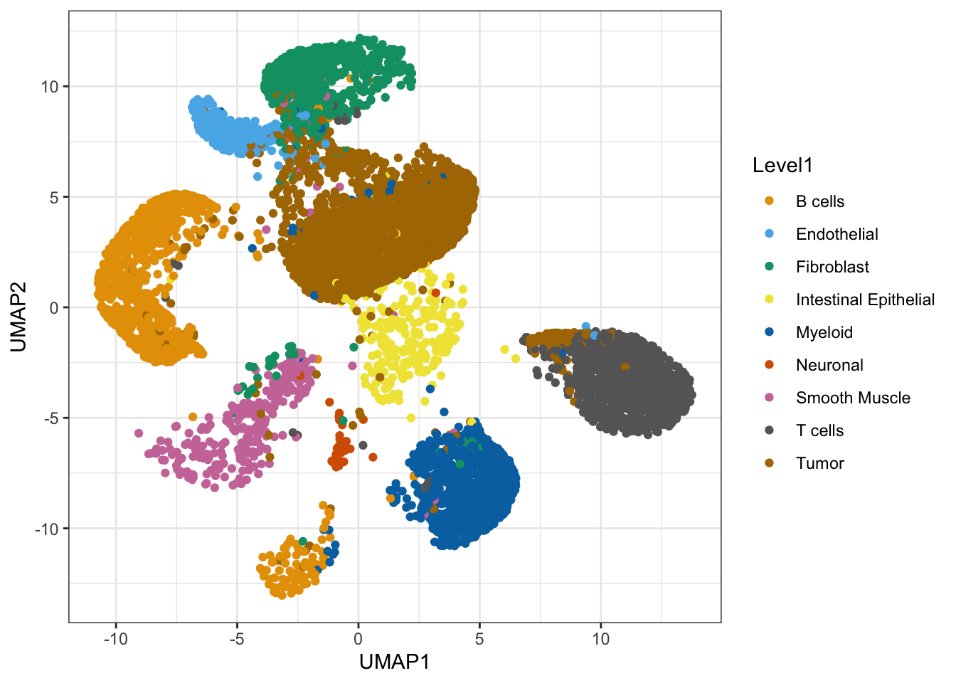

ggcells(ref.sce, aes(x = UMAP1, y=UMAP2, color=Level2)) + 
  geom_point() +
  scale_colour_manual(values = ditto_colors) + 
  theme_bw()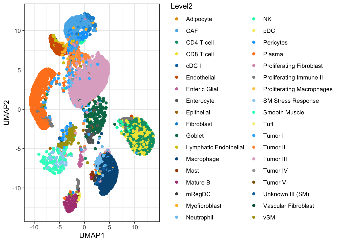

Exercise 3

What do you observe?

Answer

The cell types match the expectations based on the tissue sample we could study earlier in the course. It includes tumore cells, stromal cells and immune cells.

A few cells in the dataset could be misannotated, although this might be an impression induced by the distortion typical of dimensionality reductions like UMAP.

Perform the anotation with `SingleR`

To annotate each cell, we use the SingleR() method, which uses a correlation-based approach comparing cells from the Visium HD dataset to reference cells from the FLEX dataset with known cell-type annotation.

We will use below the highest-level annotation available. A pseudo-bulk aggregation step before the comparison allows for a better performance. We also disable the fine tuning setp for faster computation here:

table(colData(ref.sce)$Level1)


              B cells           Endothelial            Fibroblast 
                  990                   309                  1058 
Intestinal Epithelial               Myeloid              Neuronal 
                  252                  1120                    32 
        Smooth Muscle               T cells                 Tumor 
                  297                  1250                  3680

# Predict cell-type using SingleR 
pred <- SingleR(test = sfe,
                ref = ref.sce,
                labels = ref.sce$Level1,
                aggr.ref = TRUE,       
                fine.tune = FALSE,     
)
sfe$SingleR_label <- pred$pruned.labels
table(sfe$SingleR_label)


              B cells           Endothelial            Fibroblast 
                 3616                  2546                  8377 
Intestinal Epithelial               Myeloid              Neuronal 
                 5057                  2296                    34 
        Smooth Muscle               T cells                 Tumor 
                  942                   906                  9989

# visualize the predictions on the tissue slide.
plotSpatialFeature(sfe,  
                   colGeometryName = "cellSeg",
                   features = "SingleR_label")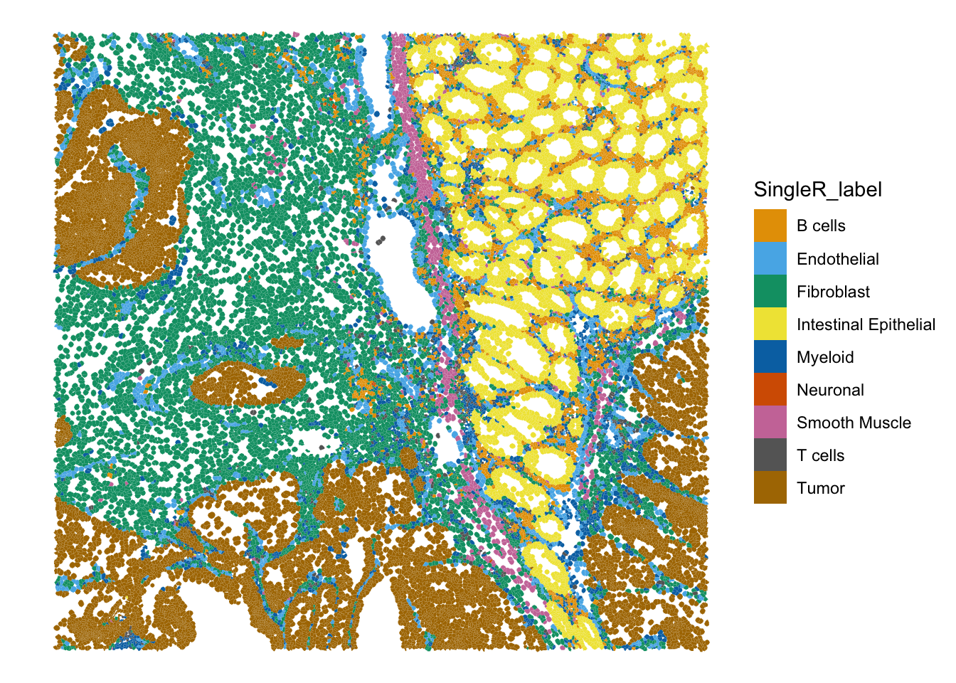

## Or on the UMAP
ggcells(sfe, aes(x = UMAP.1, y=UMAP.2, color=SingleR_label)) + 
  geom_point() +
  scale_colour_manual(values = ditto_colors) + 
  theme_bw()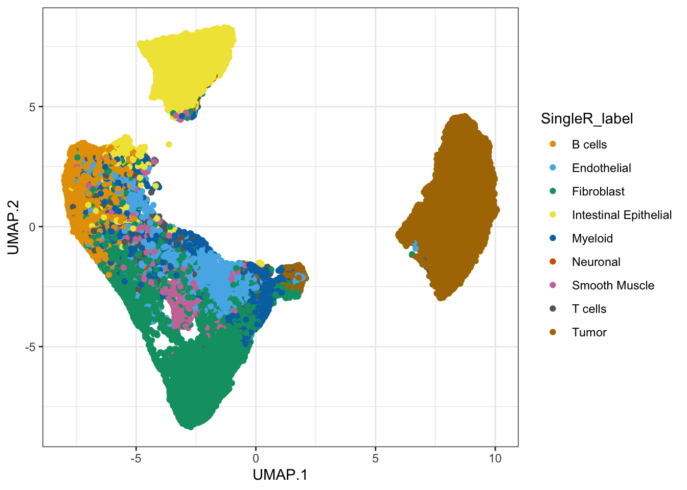

Exercise 4

What do you think about this annotation?

How do the proportions of different cell types compare to the annotated scRNA-seq dataset?

Do you identify potentially relevant biological structures? Go back to the calculated clusters and spatial domains, to see how do they match.

Try annotating the dataset with the higher-resolution cell-types lables in ref.sce$Level2

Answer

Let’s calculate the proportion of cells from each cell type:

prop.table(table(ref.sce$Level1))


              B cells           Endothelial            Fibroblast 
          0.110146862           0.034379172           0.117712506 
Intestinal Epithelial               Myeloid              Neuronal 
          0.028037383           0.124610592           0.003560303 
        Smooth Muscle               T cells                 Tumor 
          0.033044059           0.139074321           0.409434802

prop.table(table(sfe$SingleR_label))


              B cells           Endothelial            Fibroblast 
           0.10709949            0.07540799            0.24811184 
Intestinal Epithelial               Myeloid              Neuronal 
           0.14977934            0.06800344            0.00100702 
        Smooth Muscle               T cells                 Tumor 
           0.02790036            0.02683411            0.29585641

We observe a relatively higher proportion of Endothelial cells and Fibroblast in the Visium HD. Maybe such cell-types are less easily captured by the droplet-based scRNA-seq technology?

The annotation allows us to identify the different structures of the intestine mucosa very clearly, with the epithelial cells composing the intestinal villi, the smooth muscle layer, and the more scattered immune cells. In this colorectal cancer sample, the invading tumor is identified very clearly.

Let’s compare the annotation to the Leiden clustering for example:

plotSpatialFeature(sfe,  
                   colGeometryName = "cellSeg",
                   features = "SingleR_label") +
  plotSpatialFeature(sfe,  
                   colGeometryName = "cellSeg",
                   features = "Leiden")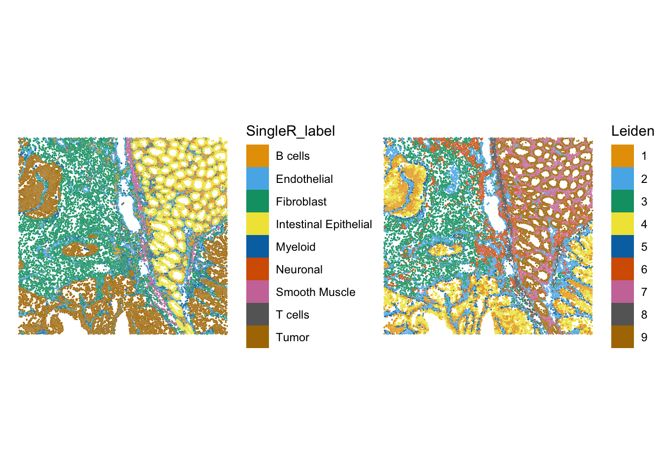

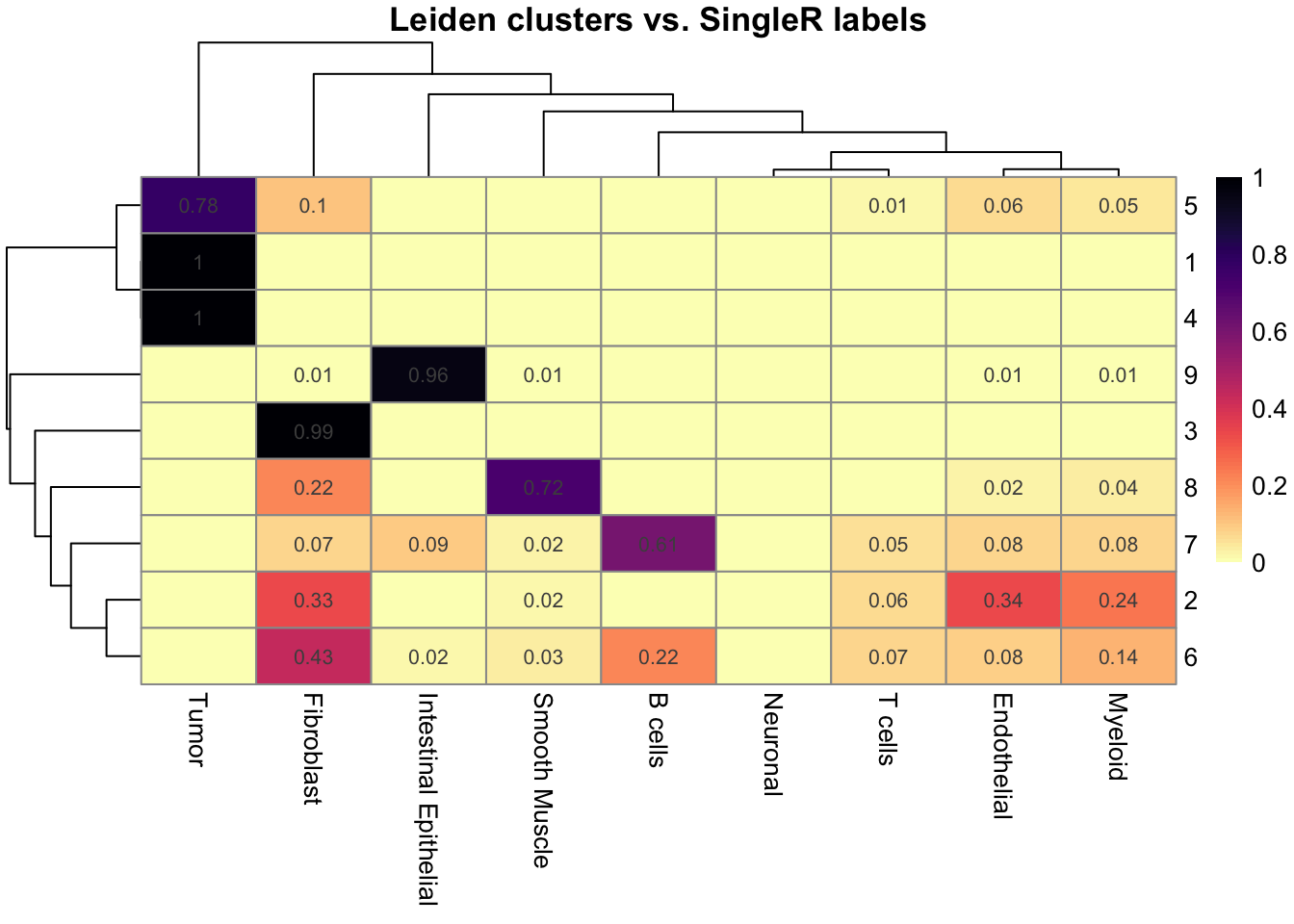
## For a more formal comparison
tab_prop <- prop.table(table(sfe$Leiden, sfe$SingleR_label), margin = 1)
## Display the proportions: round and remove 0s
num_mat <- round(tab_prop, 2)
num_mat[num_mat == 0] <- ""

pheatmap(
  tab_prop,
  cluster_rows = TRUE,
  cluster_cols = TRUE,
  color = viridis(100, option = "magma", direction = -1),
  display_numbers = num_mat,
  main = "Leiden clusters vs. SingleR labels", 
  annotation_colors = list(SingleR_label = setNames(object = ditto_colors[1:9], colnames(tab_prop)))  
)

Exercise 5: Xenium (Bonus)

Perform the same annotation task on the Xenium dataset. How do the results compare? What could be a limitation here?

Answer

One limitation of this Xenium dataset is the limited number of genes targeted by the probe panel. Some recent benchmarks seem to suggest that the classical scRNA-seq annotation methods (label-transfer methods) perform relatively well: https://link.springer.com/article/10.1186/s12859-025-06044-0

Exercise 6: RCTD (Bonus)

We ignored the fact that segmented data suffer from segmentation error, that multiple cells can overlap on the slide, and that spatial data in general suffers from local diffusion of transcripts. All these result in contamination of each cell’s transcriptome with transcripts from other cells.

It is possible to use deconvolution methods to “decontaminate” the cells. For example the RCTD method from the spacexr package (Cable et al. 2022) can be used in flag these cases and provide a principled estimate of the most likely composition. Try to run this method on our dataset, you can refer to this section of the OSTA book for guidance.

How do you interpret the results?

Answer

See the vignette here: https://raw.githack.com/dmcable/spacexr/master/vignettes/spatial-transcriptomics.html

## Install latest version from Github
BiocManager::install("dmcable/spacexr")
library(spacexr)
sort(table(ref.sce$Level2))
## We need a minimum of 25 cells for each cell type in the reference, so we'll go for Level1 here
reference <- Reference(counts(ref.sce), 
                       cell_types=setNames(factor(ref.sce$Level1), nm = colnames(ref.sce)), 
                       nUMI=colSums(counts(ref.sce)))
## Create SpatialRNA object
to_annotate <- SpatialRNA(coords=data.frame(spatialCoords(sfe)), 
                          counts=counts(sfe),
                          nUMI=colSums(counts(sfe)))
rctd_data <- create.RCTD(to_annotate, reference)

## Run RCTD
res <- run.RCTD(rctd_data, doublet_mode="doublet")
## We use here the "doublet" mode to fit at most two cell types per segmented cell, probably this is a reasonable assumption for a high-resolution technology such as Visium HD.

## Inspect results
results <- res@results
# normalize the cell type proportions to sum to 1.
norm_weights <- normalize_weights(results$weights) 
cell_type_names <- res@cell_type_info$info[[2]] #list of cell type names

# Plots the confident weights for each cell type as in full_mode (saved as 
# 'results/cell_type_weights.pdf')
plot_weights(cell_type_names, to_annotate, "./results/", norm_weights) 

## Likely "doublets"
sfe$RCTD.doublet <- NA
colData(sfe)[row.names(results$results_df), ]$RCTD.doublet <- as.character(results$results_df$spot_class)
plotSpatialFeature(sfe,  
                   colGeometryName = "cellSeg",
                   features = "RCTD.doublet") 

## Extract major cell type
sfe$RCTD.first <- NA
colData(sfe)[row.names(results$results_df), ]$RCTD.first <- as.character(results$results_df$first_type)
plotSpatialFeature(sfe,  
                   colGeometryName = "cellSeg",
                   features = "RCTD.first") 

## Plotting the normalized weights for each cell type
lapply(colnames(norm_weights), \(k) {
    colData(sfe)$foo <- NA
    colData(sfe)[row.names(norm_weights), ]$foo <- norm_weights[, k]
    plt <- plotSpatialFeature(sfe, features = "foo") + 
      scale_color_gradientn(colors=pals::jet())
    plt + ggtitle(k) + guides(fill="none")
}) |>
  wrap_plots(nrow=3)

Saving the final `SpatialFeatureExperiment` object

alabaster.sfe::saveObject(sfe, "results/day2/02.4_sfe")

Dataset loading

Download the FLEX dataset

Load the P2CRC sample

Load the annotation

Perform the anotation with SingleR

Saving the final SpatialFeatureExperiment object

Perform the anotation with `SingleR`

Saving the final `SpatialFeatureExperiment` object