Integration

Material

Exercises

library(Seurat)
seu <- readRDS("day2/seu_day2-2.rds")

Let’s have a look at the UMAP again. Although cells of different samples are shared amongst ‘clusters’, you can still see seperation within the clusters:

Seurat::DimPlot(seu, reduction = "umap")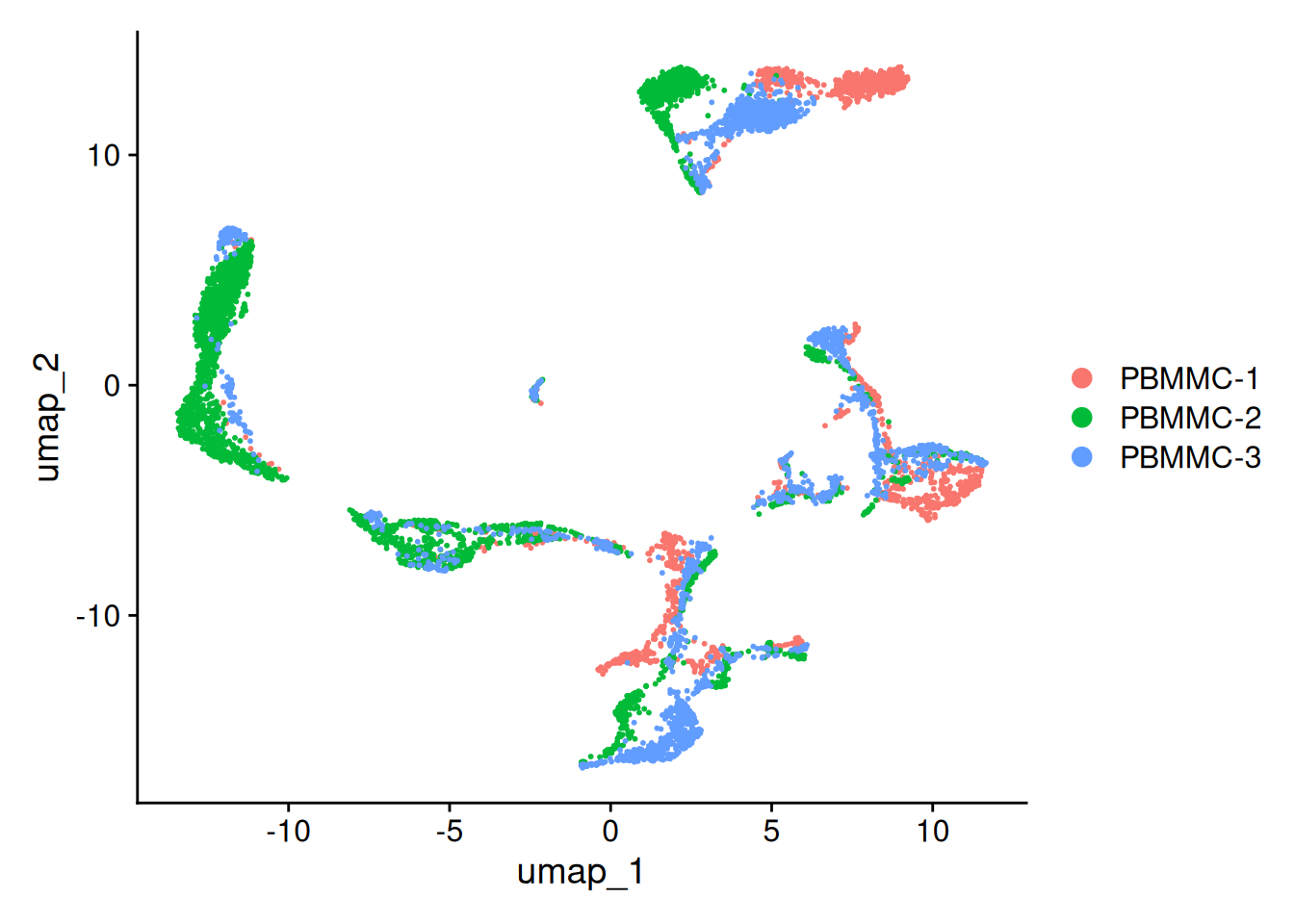

Let’s also make the function again for 3D UMAP

library(plotly)
seu <- Seurat::RunUMAP(seu, dims = 1:25, n.components = 3, reduction.name = "umap_3D")

plot_3d_umap <- function(seu,
                         reduction = "umap_3D",
                         sample_col = "orig.ident",
                         point_size = 4,
                         point_opacity = 0.5) {
  
  ## 1. Extract coordinates -------------------------------------------------
  umap_coords <- as.data.frame(Embeddings(seu, reduction = reduction))
  umap_coords$Sample <- seu@meta.data[[sample_col]]
  umap_coords$Cell   <- rownames(umap_coords)   # for hover
  
  ## 2. Build Plotly object --------------------------------------------------
  p <- plot_ly(
    data = umap_coords,
    x = ~umap3D_1, y = ~umap3D_2, z = ~umap3D_3,
    color = ~Sample,                     # default Plotly palette
    type = "scatter3d",
    mode = "markers",
    marker = list(
      size = point_size,
      opacity = point_opacity
    ),
    text = ~paste("Cell:", Cell, "<br>Sample:", Sample),
    hovertemplate = "<b>%{text}</b><extra></extra>"
  ) %>%
    layout(
      title = list(
        text = "<b>3D UMAP of Cells by Sample</b>",
        font = list(size = 18, family = "Arial, sans-serif"),
        x = 0.5, xanchor = "center", y = 0.95
      ),
      scene = list(
        xaxis = list(
          title = "<b>UMAP 1</b>", titlefont = list(size = 14),
          showgrid = TRUE, gridcolor = "rgba(200,200,200,0.5)",
          backgroundcolor = "rgba(245,245,255,0.9)",
          zerolinecolor = "rgba(100,100,100,0.3)"
        ),
        yaxis = list(
          title = "<b>UMAP 2</b>", titlefont = list(size = 14),
          showgrid = TRUE, gridcolor = "rgba(200,200,200,0.5)",
          backgroundcolor = "rgba(245,245,255,0.9)",
          zerolinecolor = "rgba(100,100,100,0.3)"
        ),
        zaxis = list(
          title = "<b>UMAP 3</b>", titlefont = list(size = 14),
          showgrid = TRUE, gridcolor = "rgba(200,200,200,0.5)",
          backgroundcolor = "rgba(245,245,255,0.9)",
          zerolinecolor = "rgba(100,100,100,0.3)"
        ),
        camera = list(eye = list(x = 1.5, y = 1.5, z = 1.5)),
        aspectmode = "cube"
      ),
      legend = list(
        title = list(text = "<b>Sample</b>", font = list(size = 12)),
        bgcolor = "rgba(255,255,255,0.8)",
        bordercolor = "gray", borderwidth = 1
      ),
      margin = list(l = 0, r = 0, t = 60, b = 0),
      paper_bgcolor = "rgba(250,250,252,1)",
      plot_bgcolor  = "rgba(250,250,252,1)"
    ) %>%
    config(
      displayModeBar = TRUE,
      displaylogo = FALSE,
      modeBarButtonsToRemove = c("sendDataToCloud", "lasso2d", "select2d")
    )
  
  return(p)
}

plot_3d_umap(seu = seu, reduction = "umap_3D", sample_col = "orig.ident")

To perform the integration, we split our object by sample, resulting into a set of layers within the RNA assay. The layers are integrated and stored in the reduction slot - in our case we call it integrated.cca. Then, we re-join the layers

seu[["RNA"]] <- split(seu[["RNA"]], f = seu$orig.ident)

seu <- Seurat::IntegrateLayers(object = seu, method = CCAIntegration,
                       orig.reduction = "pca",
                       new.reduction = "integrated.cca",
                       verbose = FALSE)

# re-join layers after integration
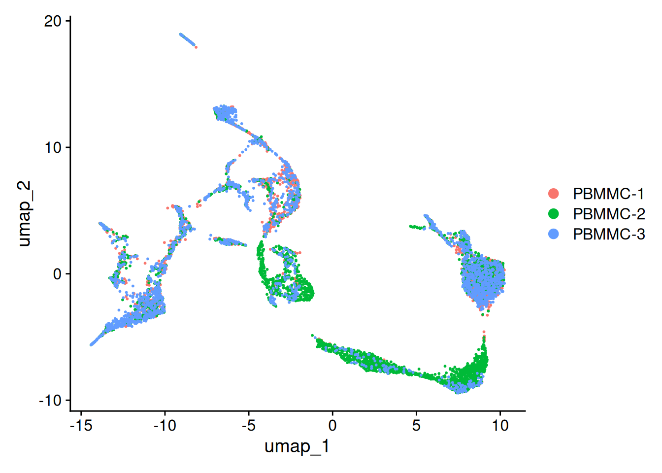
seu[["RNA"]] <- JoinLayers(seu[["RNA"]])

We can then use this new integrated matrix for clustering and visualization. Now, we can re-run and visualize the results with UMAP.

Exercise

Create the UMAP again on the integrated.cca reduction (using the function RunUMAP - set the option reduction accordingly). After that, generate the UMAP plot. Did the integration perform well?

Answer

Performing the scaling, PCA and UMAP:

seu <- RunUMAP(seu, dims = 1:30, reduction = "integrated.cca")

Plotting the UMAP:

Seurat::DimPlot(seu, reduction = "umap")

Also in 3D

seu <- RunUMAP(seu, dims = 1:30, n.components = 3, , reduction = "integrated.cca", reduction.name = "umap_3D")

13:58:22 UMAP embedding parameters a = 0.9922 b = 1.112

13:58:22 Read 6830 rows and found 30 numeric columns

13:58:22 Using Annoy for neighbor search, n_neighbors = 30

13:58:22 Building Annoy index with metric = cosine, n_trees = 50

0%   10   20   30   40   50   60   70   80   90   100%

[----|----|----|----|----|----|----|----|----|----|

**************************************************|
13:58:23 Writing NN index file to temp file /var/folders/cm/nwh7kr5n65b3m40y__9_t5hnkkqk0y/T//RtmpLREPNt/file5e9c602306e6
13:58:23 Searching Annoy index using 1 thread, search_k = 3000
13:58:24 Annoy recall = 100%
13:58:24 Commencing smooth kNN distance calibration using 1 thread with target n_neighbors = 30
13:58:24 Initializing from normalized Laplacian + noise (using RSpectra)
13:58:24 Commencing optimization for 500 epochs, with 300572 positive edges
13:58:24 Using rng type: pcg
13:58:31 Optimization finished

plot_3d_umap(seu = seu, reduction = "umap_3D", sample_col = "orig.ident")

Save the dataset and clear environment

saveRDS(seu, "day2/seu_day2-3.rds")