Setup

Material

Exercises

Login and set up

Choose one of the following:

Enrolled: if you are enrolled in a course with a teacher
Own installation: if you want to install packages on your own local Rstudio installation
Docker: if you want to use the docker image locally
renkulab.io if you want to easily deploy the environment outside the course

The account is yours for the duration of the course: the files in your home directory are only visible to you, and all R packages for the course are already installed.
For the project work, groups share files in /group_work (see Projects), and you can use an AI coding assistant: Posit Assistant in RStudio, or goose in the Terminal (see Using AI assistants with LLM packs). Do the course exercises without it.
The server, including your files, is removed after the course. Download anything you want to keep before then (in the Files pane: select files, More → Export…).

Install the required packages using renv

install.packages("renv")

renv::restore(lockfile = "https://raw.githubusercontent.com/sib-swiss/single-cell-r-training/refs/heads/master/renv.lock")

With docker, you can use exactly the same R environment as we use in the enrolled course, but than running locally. The AI coding assistants on the course server are not set up in the image (goose is not included, and Posit Assistant needs a connection to a language model of your own); see Using AI assistants with LLM packs to set one up yourself.

In the video below there’s a short tutorial on how to set up a docker container for this course. Note that you will need administrator rights, and that if you are using Windows, you need the latest version of Windows 10.

The command to run the environment required for this course looks like this (in a terminal):

Modify the script

The home directory within the container is mounted to your current directory ($PWD), if you want to change this behaviour, modify the path after -v to the working directory on your computer before running it.

docker run \
--rm \
-p 8787:8787 \
-e PASSWORD=test \
-v $PWD:/home/rstudio \
sibswiss/training-singlecell-rstudio:2026.3

If this command has run successfully, approach Rstudio server like this:

http://localhost:8787

Copy this URL into your browser. If you used the snippet above, the credentials will be:

Username: rstudio
Password: test

Great! Now you will be able to use Rstudio with all required installations.

About the options

The option -v mounts a local directory in your computer to the directory /home/rstudio in the docker container (‘rstudio’ is the default user for Rstudio containers). In that way, you have files available both in the container and on your computer. Use this directory on your computer. Change the first path to a path on your computer that you want to use as a working directory.

The part sibswiss/training-singlecell-rstudio:2026.3 is the image we are going to load into the container. The image contains all the information about software and dependencies needed for this course. When you run this command for the first time it will download the image. Once it’s on your computer, it will start immediately.

To simply run the environment, you can use renku. You can find the repository (including the image) here: https://renkulab.io/projects/geert.vangeest/single-cell-training/.

Create a project

Now that you have access to an environment with the required installations, we will set up a project in a new directory. On the top right choose the button Project (None) and select New Project…

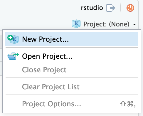
Continue by choosing New Directory

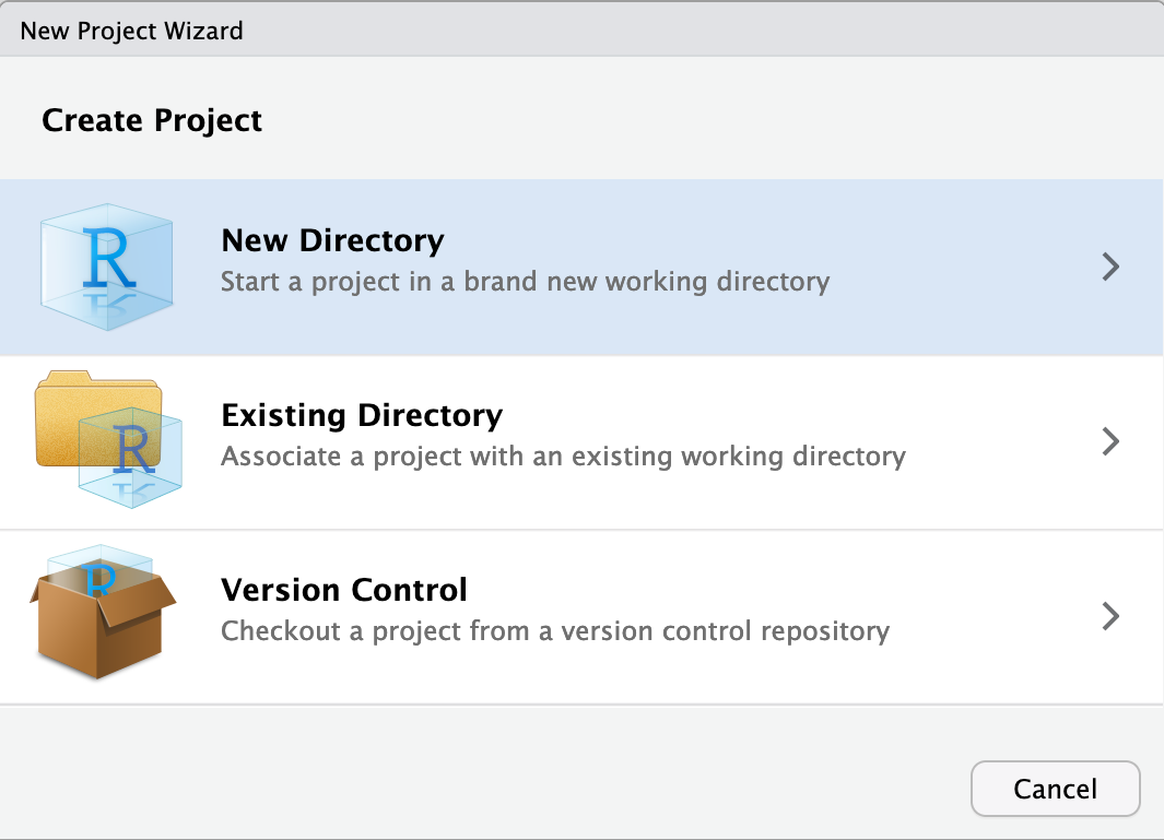
As project type select New Project

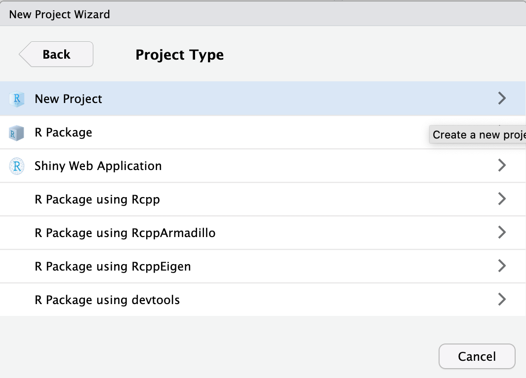
Finally, type in the project name. This should be single_cell_course. Finish by clicking Create Project.

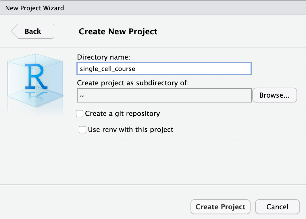
Now that we have setup a project and a project directory (it is in ~/single_cell_course), we can download the data that is required for this course.

To download and extract the dataset, copy-paste these commands in the Console tab:

download.file(
  url = "https://single-cell-transcriptomics.s3.eu-central-1.amazonaws.com/course_data.tar.gz",
  destfile = "course_data.tar.gz"
)
untar("course_data.tar.gz")

file.remove("course_data.tar.gz")

[1] TRUE

If on Windows

If you’re using Windows, you can directly open the link in your browser, and downloading will start automatically. Unpack the tar.gz file in the directory where you want to work in during the course.

Have a look at the data directory you have downloaded. It should contain the following:

course_data
├── count_matrices
│   ├── ETV6-RUNX1_1
│   │   └── outs
│   │       └── filtered_feature_bc_matrix
│   │           ├── barcodes.tsv.gz
│   │           ├── features.tsv.gz
│   │           └── matrix.mtx.gz
│   ├── ETV6-RUNX1_2
│   │   └── outs
│   │       └── filtered_feature_bc_matrix
│   │           ├── barcodes.tsv.gz
│   │           ├── features.tsv.gz
│   │           └── matrix.mtx.gz
│   ├── ETV6-RUNX1_3
│   │   └── outs
│   │       └── filtered_feature_bc_matrix
│   │           ├── barcodes.tsv.gz
│   │           ├── features.tsv.gz
│   │           └── matrix.mtx.gz
│   ├── PBMMC_1
│   │   └── outs
│   │       └── filtered_feature_bc_matrix
│   │           ├── barcodes.tsv.gz
│   │           ├── features.tsv.gz
│   │           └── matrix.mtx.gz
│   ├── PBMMC_2
│   │   └── outs
│   │       └── filtered_feature_bc_matrix
│   │           ├── barcodes.tsv.gz
│   │           ├── features.tsv.gz
│   │           └── matrix.mtx.gz
│   └── PBMMC_3
│       └── outs
│           └── filtered_feature_bc_matrix
│               ├── barcodes.tsv.gz
│               ├── features.tsv.gz
│               └── matrix.mtx.gz
└── reads
    ├── ETV6-RUNX1_1_S1_L001_I1_001.fastq.gz
    ├── ETV6-RUNX1_1_S1_L001_R1_001.fastq.gz
    └── ETV6-RUNX1_1_S1_L001_R2_001.fastq.gz

20 directories, 21 files

This data comes from:

Caron M, St-Onge P, Sontag T, Wang YC, Richer C, Ragoussis I, et al. Single-cell analysis of childhood leukemia reveals a link between developmental states and ribosomal protein expression as a source of intra-individual heterogeneity. Scientific Reports. 2020;10:1–12. Available from: http://dx.doi.org/10.1038/s41598-020-64929-x

About the Course Dataset & How It Was Generated

To understand the data you are about to analyze in R, here is a quick overview of its origin and processing:

Biological Source: The dataset comprises human peripheral blood mononuclear cells (PBMCs) and bone marrow samples from healthy donors and pediatric patients with ETV6-RUNX1 acute lymphoblastic leukemia.
Wet-Lab Generation (10x Genomics):
- Single-Cell Partitioning: Cell suspensions were captured using 10x Genomics Chromium microfluidic chips, encapsulating single cells into oil droplets (GEMs) along with barcoded gel beads.
- Barcoding & UMIs: Each cell received a unique 16-base cell barcode, and individual mRNA molecules were tagged with a Unique Molecular Identifier (UMI) to eliminate PCR amplification bias.
- Sequencing: Libraries were sequenced on Illumina platforms, producing raw FASTQ read files (found in course_data/reads/).
Computational Processing & Course Subsetting:
- Raw reads were aligned to the human reference genome using Cell Ranger, generating count matrices.
- Curious how the course data was prepared? You can inspect the automated pipeline scripts in the course repository under scripts/generate_dataset/.

We will use the reads to showcase the use of cellranger count. The directory contains only reads from chromosome 21 and 22 of one sample (ETV6-RUNX1_1). The count matrices are output of cellranger count, and we will use those for the other exercises in R.

Clear your environment:

gc()