Trajectory and pseudotime analysis

Learning outcomes

After having completed this chapter you will be able to:

Understand the biological rationale and concepts behind trajectory inference and pseudotime analysis.
Convert a clustered Seurat object into a Monocle3 cell_data_set object.
Pre-process, reduce dimensions, and learn a principal graph trajectory from single-cell RNA-seq data.
Order cells along pseudotime starting from progenitor/root populations based on cluster annotations.
Identify and plot genes whose expression changes dynamically along a developmental or differentiation trajectory.

Introduction to Trajectory and Pseudotime Analysis

While clustering and cell annotation group cells into discrete cell types or states, biological processes such as cellular differentiation, activation, or development are often continuous dynamic processes.

Trajectory inference and pseudotime analysis order cells along one or more continuous paths (lineages) based on similarities in their gene expression profiles. By building on top of our pre-computed Seurat clusters, we can easily identify progenitor cell populations, learn the underlying graph topology, and assign each cell a pseudotime value representing its relative progression along the biological process.

Exercises

Advanced Exercise: Package Installation

Since this is an advanced exercise, required packages like monocle3, leidenbase, and BPCells are not installed by default in the standard course environment. If you wish to install them, you can run the following code:

renv::install(c("SingleCellExperiment", "scater", "ggbeeswarm", "remotes", "devtools"))

# For monocle3:
remotes::install_github("bnprks/BPCells/r")
renv::install("cole-trapnell-lab/monocle3")

1. Load Required Packages and Clustered Data

First, load the required packages and the clustered Seurat object (seu_day2-4.rds) created during the clustering step:

library(Seurat)
library(monocle3)
library(ggplot2)

# Load clustered Seurat object from day 2 clustering step
seu <- readRDS("day2/seu_day2-4.rds")

Let’s inspect the UMAP visualization with our cluster annotations:

Seurat::DimPlot(seu, reduction = "umap", label = TRUE)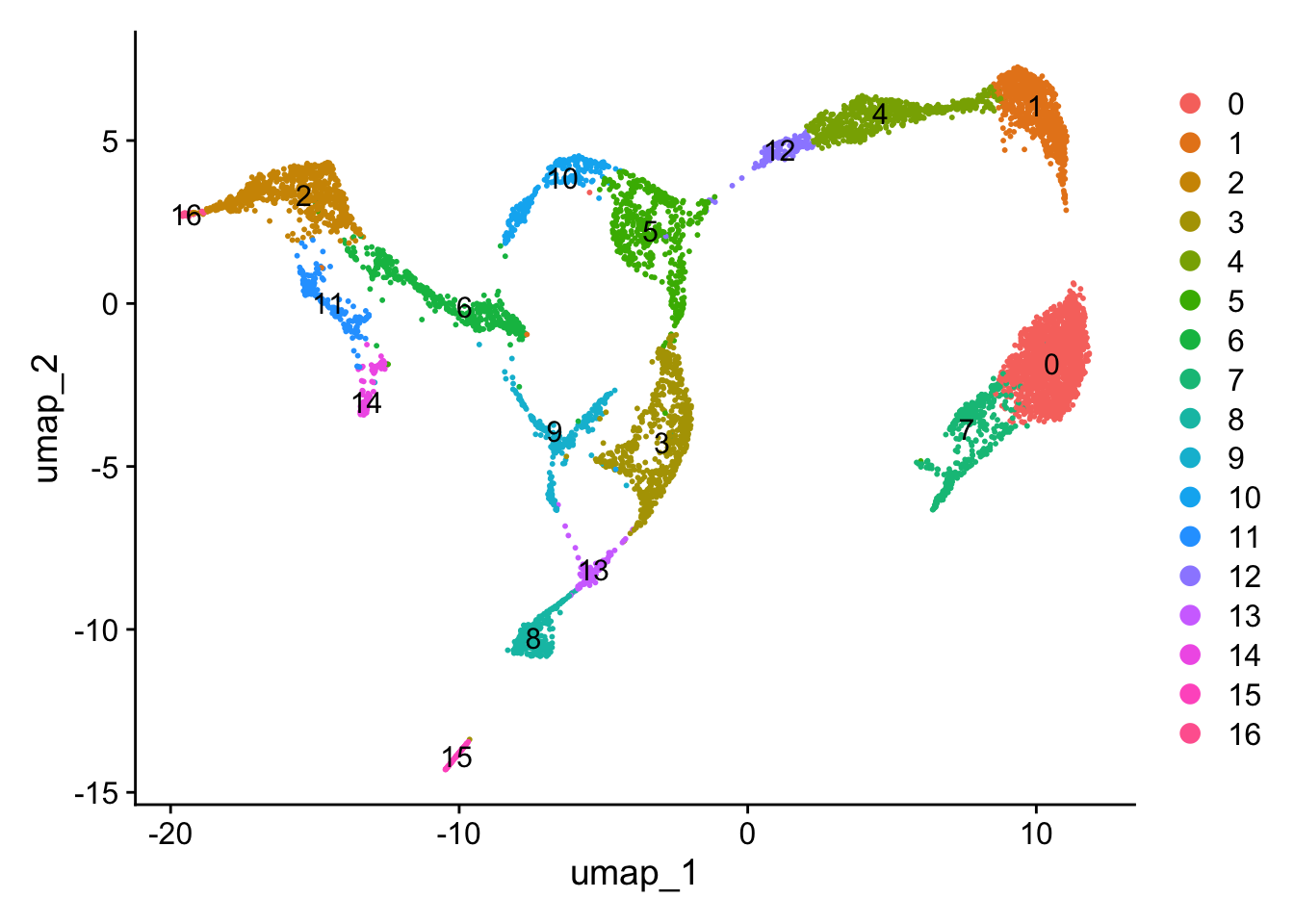

2. Converting Seurat Object to Monocle3 Object

monocle3 operates on objects of class cell_data_set. We construct a Monocle3 object directly from our Seurat object’s count matrix, cell metadata (including cluster assignments), and gene metadata.

# Create gene metadata data.frame
feature_names <- data.frame(gene_short_name = rownames(seu), row.names = rownames(seu))

# Initialize monocle3 object from Seurat count table and metadata
seu_monocl <- new_cell_data_set(
  expression_data = GetAssayData(seu, layer = "counts"),
  cell_metadata = seu@meta.data,
  gene_metadata = feature_names
)

3. Pre-processing and Dimensionality Reduction in Monocle3

Just like Seurat, Monocle3 requires normalization, scaling, and dimensionality reduction. We use preprocess_cds() and reduce_dimension():

# Pre-process the CDS object
seu_monocl <- preprocess_cds(seu_monocl, num_dim = 30)

# Reduce dimensions using UMAP
seu_monocl <- reduce_dimension(seu_monocl, reduction_method = "UMAP")

No preprocess_method specified, using preprocess_method = 'PCA'

We can visualize the cells in Monocle3 UMAP space, colored by Seurat cluster IDs:

plot_cells(seu_monocl, 
           color_cells_by = "seurat_clusters", 
           cell_size = 1, 
           show_trajectory_graph = FALSE)

Warning: `aes_string()` was deprecated in ggplot2 3.0.0.
ℹ Please use tidy evaluation idioms with `aes()`.
ℹ See also `vignette("ggplot2-in-packages")` for more information.
ℹ The deprecated feature was likely used in the monocle3 package.
  Please report the issue to the authors.

Warning: The `size` argument of `element_line()` is deprecated as of ggplot2 3.4.0.
ℹ Please use the `linewidth` argument instead.
ℹ The deprecated feature was likely used in the monocle3 package.
  Please report the issue to the authors.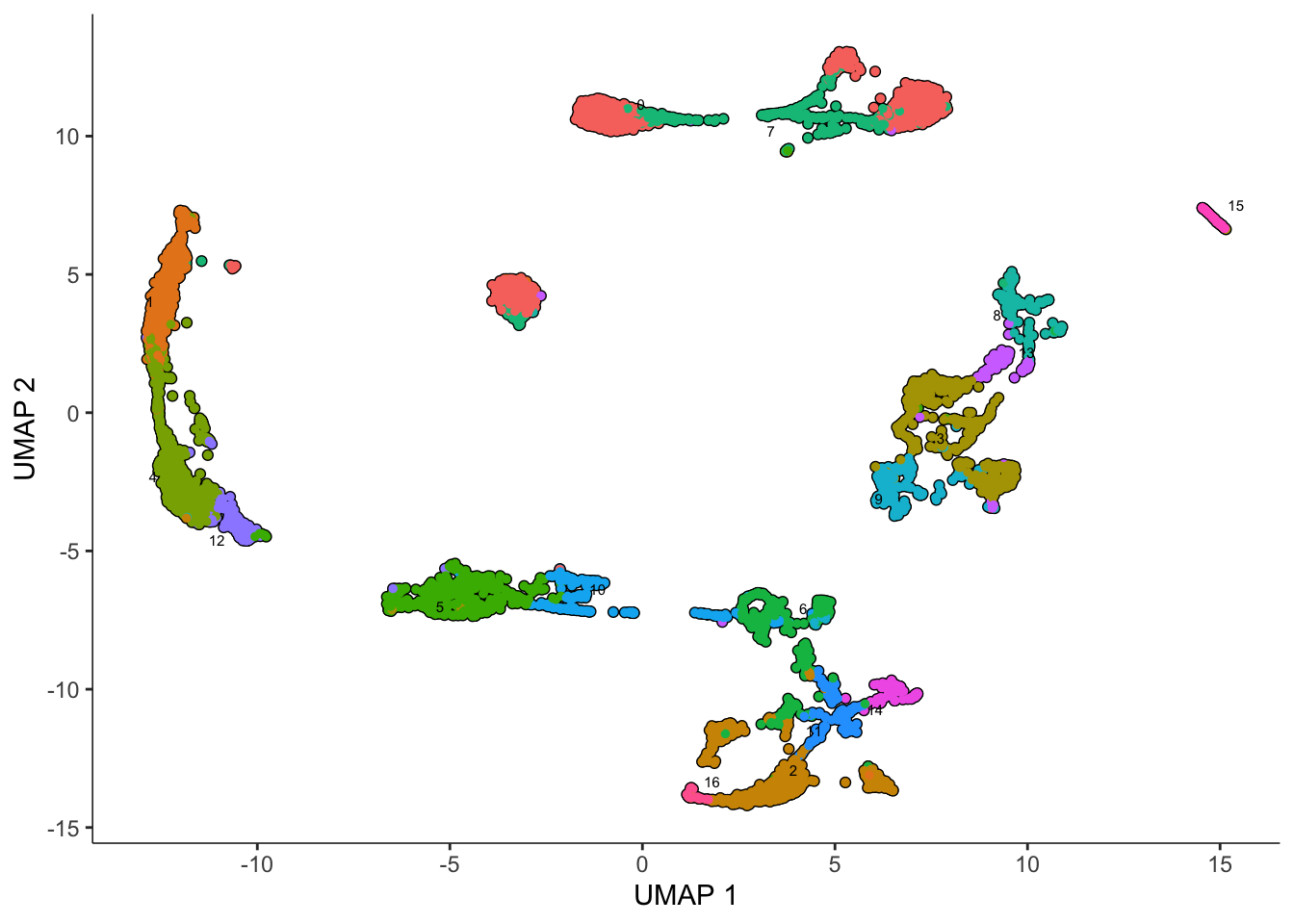

4. Clustering and Learning the Trajectory Graph

Monocle3 uses its own clustering algorithm to partition cells into communities, which are then connected by learn_graph() to infer the principal trajectory graph.

# Cluster cells using monocle3
seu_monocl <- cluster_cells(seu_monocl, resolution = 0.00025)

# Learn the principal graph trajectory
seu_monocl <- learn_graph(seu_monocl)


  |                                                                            
  |                                                                      |   0%
  |                                                                            
  |======================================================================| 100%

  |                                                                            
  |                                                                      |   0%
  |                                                                            
  |======================================================================| 100%

  |                                                                            
  |                                                                      |   0%
  |                                                                            
  |======================================================================| 100%

  |                                                                            
  |                                                                      |   0%
  |                                                                            
  |======================================================================| 100%

  |                                                                            
  |                                                                      |   0%
  |                                                                            
  |======================================================================| 100%

  |                                                                            
  |                                                                      |   0%
  |                                                                            
  |======================================================================| 100%

Warning in cluster_cells_make_graph(data = data, weight = weight, cell_names = cell_names, : The nearest neighbors includes the point itself, k must be smaller than
the total number of points - 1 (all other points) - 1 (itself)! Total number of points is 21

Warning in min(data_df$weight[data_df$weight > 0]): no non-missing arguments to
min; returning Inf

Visualize the inferred trajectory graph over the UMAP:

plot_cells(seu_monocl,
           color_cells_by = "seurat_clusters",
           label_cell_groups = FALSE,
           label_leaves = TRUE,
           label_branch_points = TRUE,
           graph_label_size = 1.5,
           cell_size = 1)

Warning: Using `size` aesthetic for lines was deprecated in ggplot2 3.4.0.
ℹ Please use `linewidth` instead.
ℹ The deprecated feature was likely used in the monocle3 package.
  Please report the issue to the authors.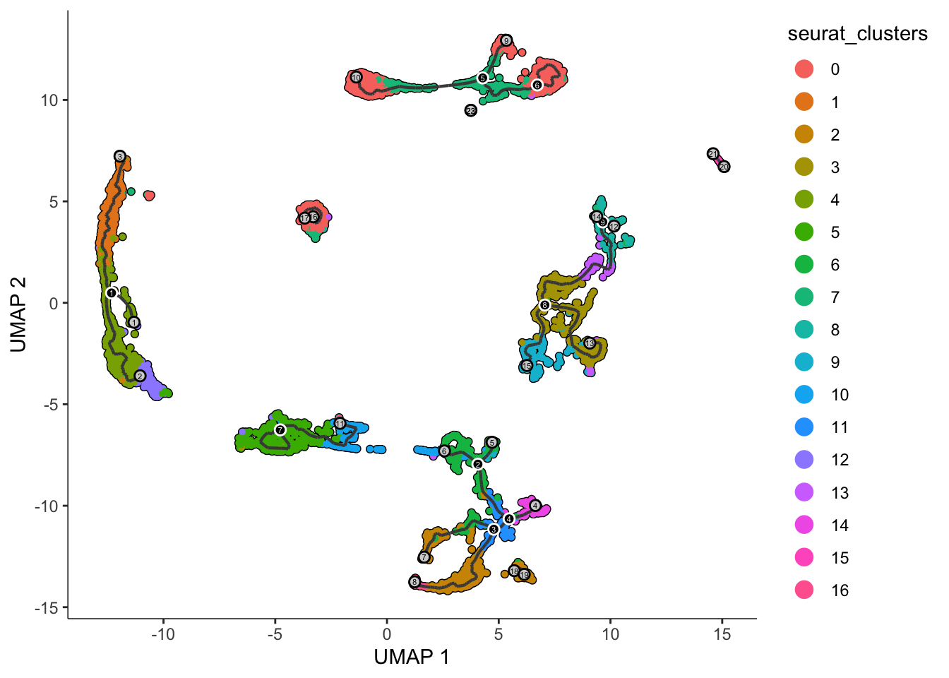

5. Ordering Cells in Pseudotime

To calculate pseudotime, we define a starting point (root node) corresponding to progenitor or stem-like cells (informed by our cluster annotations).

Using order_cells(), you can interactively select root nodes or specify them programmatically:

# Interactive root selection:
seu_monocl <- order_cells(seu_monocl)

Once the root nodes are selected, cells are ordered along pseudotime from the root:

plot_cells(seu_monocl,
           color_cells_by = "pseudotime",
           label_cell_groups = FALSE,
           label_leaves = FALSE,
           label_branch_points = FALSE,
           graph_label_size = 1.5,
           cell_size = 1)

6. Finding Genes Dynamic Along Pseudotime

To identify genes whose expression changes significantly across the trajectory, we run a graph autocorrelation test (graph_test()) on the principal graph:

pr_test <- graph_test(seu_monocl, 
                      neighbor_graph = "principal_graph", 
                      cores = 4)

We can order the results by test statistic (e.g., Moran’s I) to find the top dynamic genes, and plot their expression trends along pseudotime using plot_genes_in_pseudotime().