docker run \
--rm \
-p 8787:8787 \
-e PASSWORD=test \
-v $PWD:/home/rstudio \
geertvangeest/single-cell-rstudio:latestSetup
Material
Exercises
Login and set up
Choose one of the following:
- Enrolled: if you are enrolled in a course with a teacher
- Own installation: if you want to install packages on your own local Rstudio installation
- Docker: if you want to use the docker image locally
- renkulab.io if you want to easily deploy the environment outside the course
Log in to Rstudio server with the provided link, username and password.
Install the required packages using the script install_packages.R
With docker, you can use exactly the same environment as we use in the enrolled course, but than running locally.
In the video below there’s a short tutorial on how to set up a docker container for this course. Note that you will need administrator rights, and that if you are using Windows, you need the latest version of Windows 10.
The command to run the environment required for this course looks like this (in a terminal):
Modify the script
The home directory within the container is mounted to your current directory ($PWD), if you want to change this behaviour, modify the path after -v to the working directory on your computer before running it.
If this command has run successfully, approach Rstudio server like this:
http://localhost:8787Copy this URL into your browser. If you used the snippet above, the credentials will be:
-
Username:
rstudio -
Password:
test
Great! Now you will be able to use Rstudio with all required installations.
About the options
The option -v mounts a local directory in your computer to the directory /home/rstudio in the docker container (‘rstudio’ is the default user for Rstudio containers). In that way, you have files available both in the container and on your computer. Use this directory on your computer. Change the first path to a path on your computer that you want to use as a working directory.
The part geertvangeest/single-cell-rstudio:latest is the image we are going to load into the container. The image contains all the information about software and dependencies needed for this course. When you run this command for the first time it will download the image. Once it’s on your computer, it will start immediately.
To simply run the environment, you can use renku. You can find the repository (including the image) here: https://renkulab.io/projects/geert.vangeest/single-cell-training/.
Create a project
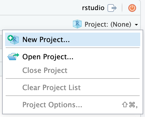
Now that you have access to an environment with the required installations, we will set up a project in a new directory. On the top right choose the button Project (None) and select New Project…
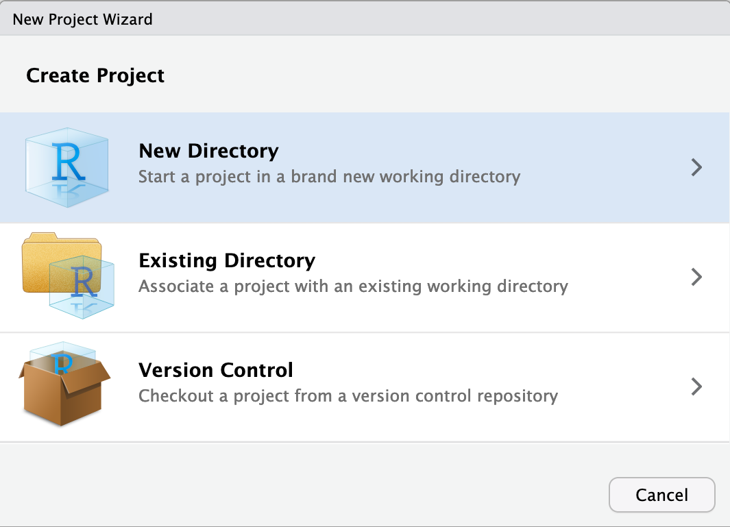
Continue by choosing New Directory
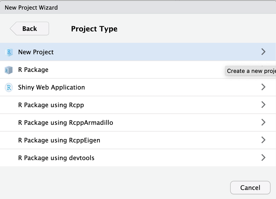
As project type select New Project
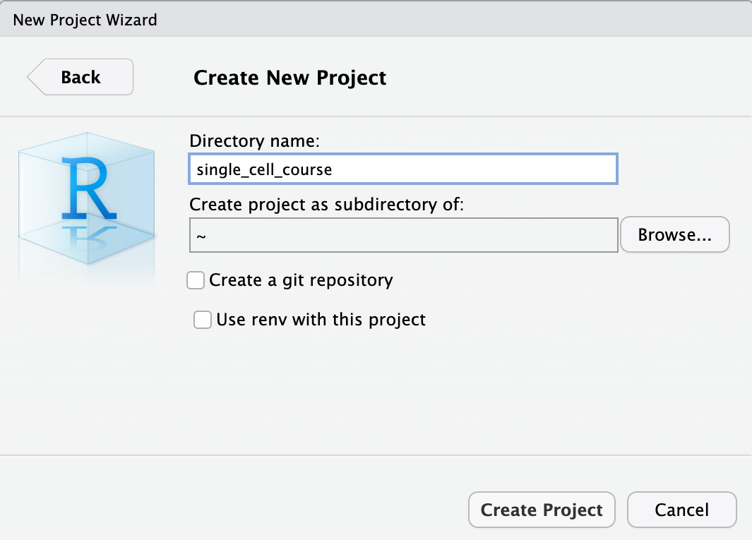
Finally, type in the project name. This should be single_cell_course. Finish by clicking Create Project.
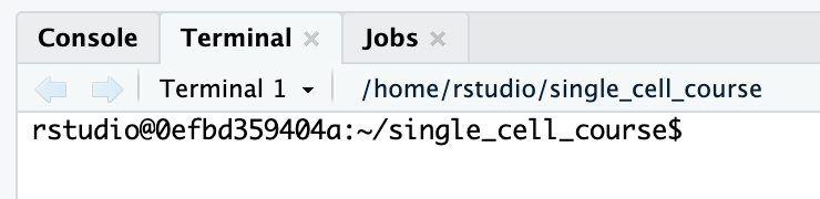
Now that we have setup a project and a project directory (it is in /home/rstudio/single_cell_course), we can download the data that is required for this course. We will use the built-in terminal of Rstudio. To do this, select the Terminal tab:
Downloading the course data
To download and extract the dataset, copy-paste these commands inside the terminal tab:
wget https://single-cell-transcriptomics.s3.eu-central-1.amazonaws.com/course_data.tar.gz
tar -xvf course_data.tar.gz
rm course_data.tar.gz
If on Windows
If you’re using Windows, you can directly open the link in your browser, and downloading will start automatically. Unpack the tar.gz file in the directory where you want to work in during the course.
Have a look at the data directory you have downloaded. It should contain the following:
course_data
├── count_matrices
│   ├── ETV6-RUNX1_1
│   │   └── outs
│   │       └── filtered_feature_bc_matrix
│   │           ├── barcodes.tsv.gz
│   │           ├── features.tsv.gz
│   │           └── matrix.mtx.gz
│   ├── ETV6-RUNX1_2
│   │   └── outs
│   │       └── filtered_feature_bc_matrix
│   │           ├── barcodes.tsv.gz
│   │           ├── features.tsv.gz
│   │           └── matrix.mtx.gz
│   ├── ETV6-RUNX1_3
│   │   └── outs
│   │       └── filtered_feature_bc_matrix
│   │           ├── barcodes.tsv.gz
│   │           ├── features.tsv.gz
│   │           └── matrix.mtx.gz
│   ├── PBMMC_1
│   │   └── outs
│   │       └── filtered_feature_bc_matrix
│   │           ├── barcodes.tsv.gz
│   │           ├── features.tsv.gz
│   │           └── matrix.mtx.gz
│   ├── PBMMC_2
│   │   └── outs
│   │       └── filtered_feature_bc_matrix
│   │           ├── barcodes.tsv.gz
│   │           ├── features.tsv.gz
│   │           └── matrix.mtx.gz
│   └── PBMMC_3
│       └── outs
│           └── filtered_feature_bc_matrix
│               ├── barcodes.tsv.gz
│               ├── features.tsv.gz
│               └── matrix.mtx.gz
└── reads
    ├── ETV6-RUNX1_1_S1_L001_I1_001.fastq.gz
    ├── ETV6-RUNX1_1_S1_L001_R1_001.fastq.gz
    └── ETV6-RUNX1_1_S1_L001_R2_001.fastq.gz

20 directories, 21 files
This data comes from:
Caron M, St-Onge P, Sontag T, Wang YC, Richer C, Ragoussis I, et al. Single-cell analysis of childhood leukemia reveals a link between developmental states and ribosomal protein expression as a source of intra-individual heterogeneity. Scientific Reports. 2020;10:1–12. Available from: http://dx.doi.org/10.1038/s41598-020-64929-x
We will use the reads to showcase the use of cellranger count. The directory contains only reads from chromosome 21 and 22 of one sample (ETV6-RUNX1_1). The count matrices are output of cellranger count, and we will use those for the other exercises in R.