seu <- readRDS("seu_day2-4.rds")Differential gene expression
Material
- More information on pseudobulk analysis
- Muscat for pseudobulk DGE.
- Paper on the robustness of different differential expression analysis methods
Exercises
Find all markers for each cluster
Load the seu dataset you have created yesterday:
And load the following packages (install them if they are missing):
The function FindAllMarkers performs a Wilcoxon plot to determine the genes differentially expressed between each cluster and the rest of the cells. Other types of tests than the Wilcoxon test are available. Check it out by running ?Seurat::FindAllMarkers.
Now run analysis:
de_genes <- Seurat::FindAllMarkers(seu, min.pct = 0.25,
only.pos = TRUE)Subset the table to only keep the significant genes, and you can save it as a csv file if you wish to explore it further. Then extract the top 3 markers per cluster:
And generate e.g. a dotplot:
dittoSeq::dittoDotPlot(seu,
vars = unique(top_specific_markers$gene),
group.by = "RNA_snn_res.0.3")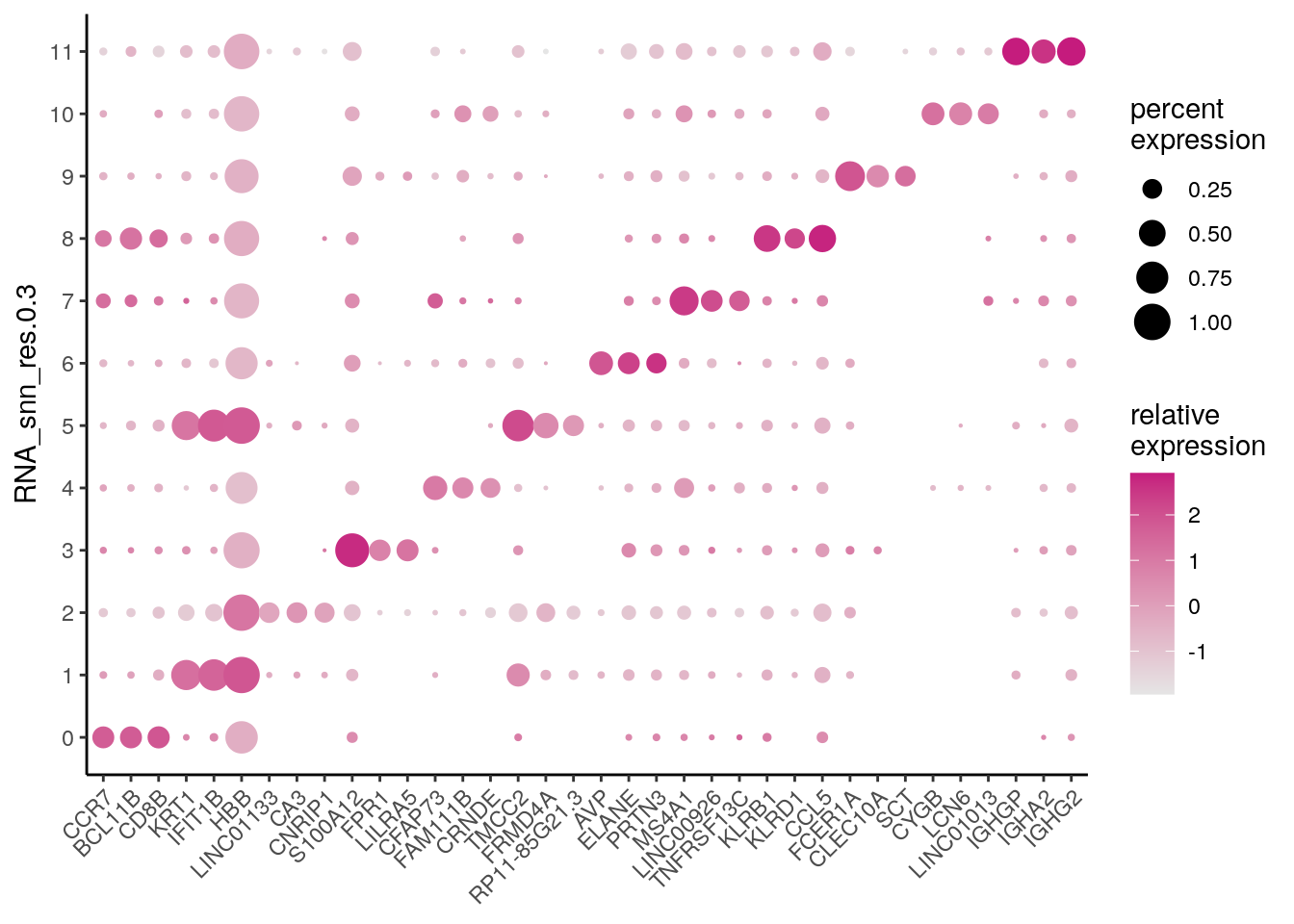
Exercise
What are significant marker genes in cluster 0 and 8? Are the T cell genes in there?
You can re-load the vector with immune genes with:
tcell_genes <- c("IL7R", "LTB", "TRAC", "CD3D")
Answer
| p_val | avg_log2FC | pct.1 | pct.2 | p_val_adj | cluster | gene | |
|---|---|---|---|---|---|---|---|
| CD3D | 0 | 2.9050191 | 0.770 | 0.227 | 0 | 0 | CD3D |
| TRAC | 0 | 2.5859745 | 0.627 | 0.202 | 0 | 0 | TRAC |
| LTB | 0 | 1.8698016 | 0.759 | 0.395 | 0 | 0 | LTB |
| IL7R | 0 | 2.8974760 | 0.438 | 0.114 | 0 | 0 | IL7R |
| LTB1 | 0 | 1.3878665 | 0.678 | 0.465 | 0 | 7 | LTB |
| TRAC1 | 0 | 2.3761801 | 0.744 | 0.274 | 0 | 8 | TRAC |
| CD3D1 | 0 | 2.1009702 | 0.799 | 0.325 | 0 | 8 | CD3D |
| LTB2 | 0 | 1.8673679 | 0.761 | 0.461 | 0 | 8 | LTB |
| IL7R1 | 0 | 1.8831338 | 0.460 | 0.172 | 0 | 8 | IL7R |
| LTB3 | 0 | 0.9176413 | 0.749 | 0.466 | 0 | 10 | LTB |
So, yes, the T-cell genes are highly significant markers for cluster 0 and 8.
Differential expression between groups of cells
The FindMarkers function allows to test for differential gene expression analysis specifically between 2 groups of cells, i.e. perform pairwise comparisons, eg between cells of cluster 0 vs cluster 2, or between cells annotated as T-cells and B-cells.
First we can set the default cell identity to the cell types defined by SingleR:
seu <- Seurat::SetIdent(seu, value = "SingleR_annot")Run the differential gene expression analysis and subset the table to keep the significant genes:
deg_cd8_cd4 <- Seurat::FindMarkers(seu,
ident.1 = "CD8+ T cells",
ident.2 = "CD4+ T cells",
group.by = seu$SingleR_annot,
test.use = "wilcox")
deg_cd8_cd4 <- subset(deg_cd8_cd4, deg_cd8_cd4$p_val_adj<0.05)
Exercise
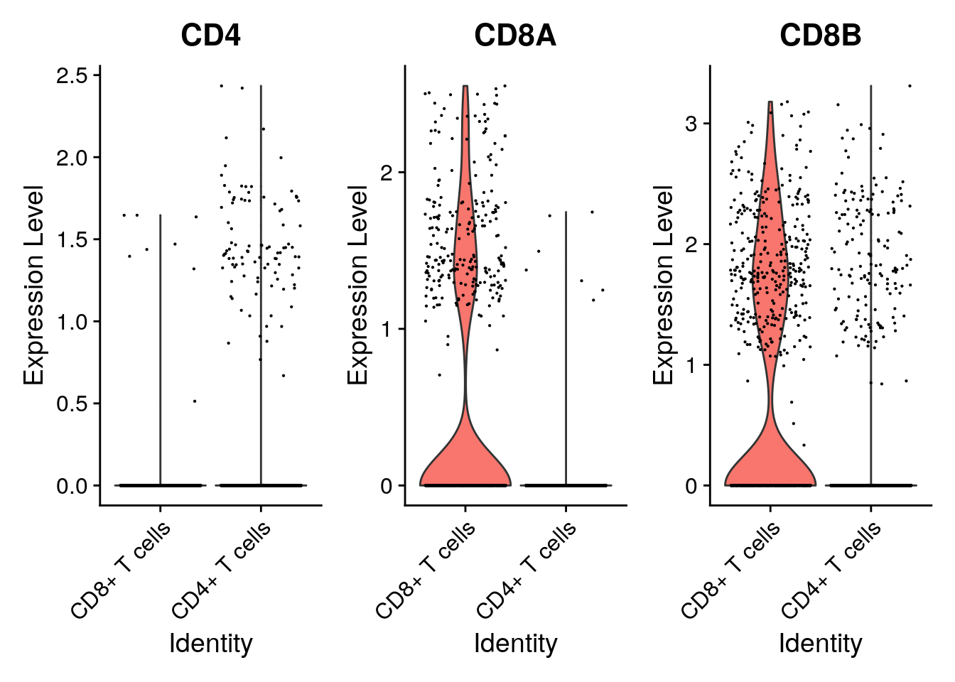
Are CD8A, CD8B and CD4 in there? What does the sign (i.e. positive or negative) mean in the log fold change values? Are they according to the CD8+ and CD4+ annotations? Check your answer by generating a violin plot of a top differentially expressed gene.
Answer
You can check out the results with:
View(deg_cd8_cd4)| p_val | avg_log2FC | pct.1 | pct.2 | p_val_adj | |
|---|---|---|---|---|---|
| CD8A | 0.0e+00 | 5.8036617 | 0.336 | 0.008 | 0.0000000 |
| CTSW | 0.0e+00 | 3.4118773 | 0.276 | 0.030 | 0.0000000 |
| CCL5 | 0.0e+00 | 4.2922622 | 0.285 | 0.062 | 0.0000000 |
| CD8B | 0.0e+00 | 1.3123538 | 0.470 | 0.178 | 0.0000000 |
| NKG7 | 0.0e+00 | 4.5376500 | 0.225 | 0.037 | 0.0000000 |
| CST7 | 0.0e+00 | 4.4123574 | 0.143 | 0.012 | 0.0000000 |
| GZMA | 0.0e+00 | 3.8501654 | 0.169 | 0.025 | 0.0000000 |
| TRGC2 | 0.0e+00 | 3.4931638 | 0.144 | 0.018 | 0.0000000 |
| RPS27 | 0.0e+00 | -0.1820605 | 1.000 | 1.000 | 0.0000000 |
| KLRD1 | 0.0e+00 | 4.3589947 | 0.108 | 0.008 | 0.0000000 |
| ID2 | 0.0e+00 | 0.8632969 | 0.565 | 0.353 | 0.0000000 |
| GZMK | 0.0e+00 | 3.0113231 | 0.130 | 0.022 | 0.0000000 |
| HCST | 0.0e+00 | 0.7949700 | 0.681 | 0.495 | 0.0000000 |
| MT-CO1 | 0.0e+00 | 0.3243268 | 0.989 | 0.979 | 0.0000000 |
| TRGC1 | 0.0e+00 | 3.6853476 | 0.110 | 0.013 | 0.0000000 |
| FHIT | 0.0e+00 | -1.6706990 | 0.110 | 0.273 | 0.0000000 |
| RP11-291B21.2 | 0.0e+00 | 1.3507107 | 0.222 | 0.077 | 0.0000000 |
| MT-ND4 | 0.0e+00 | 0.3226206 | 0.963 | 0.932 | 0.0000000 |
| CD4 | 0.0e+00 | -3.3247772 | 0.011 | 0.105 | 0.0000000 |
| MT-CO2 | 0.0e+00 | 0.2401784 | 0.993 | 0.995 | 0.0000000 |
| TRDC | 0.0e+00 | 2.6894608 | 0.105 | 0.019 | 0.0000000 |
| CRTAM | 0.0e+00 | 3.7124154 | 0.068 | 0.003 | 0.0000000 |
| PECAM1 | 0.0e+00 | 2.6701767 | 0.096 | 0.015 | 0.0000000 |
| LYAR | 0.0e+00 | 1.6580580 | 0.198 | 0.076 | 0.0000000 |
| GZMH | 0.0e+00 | 4.8543018 | 0.067 | 0.003 | 0.0000000 |
| PRF1 | 0.0e+00 | 2.8596139 | 0.099 | 0.018 | 0.0000000 |
| ACTB | 0.0e+00 | 0.3093718 | 0.965 | 0.925 | 0.0000000 |
| AC092580.4 | 0.0e+00 | 1.3359936 | 0.173 | 0.061 | 0.0000000 |
| CCL4 | 0.0e+00 | 3.7724347 | 0.118 | 0.031 | 0.0000001 |
| RPS27A | 0.0e+00 | -0.1605123 | 1.000 | 1.000 | 0.0000001 |
| RPL11 | 0.0e+00 | -0.1685948 | 1.000 | 1.000 | 0.0000002 |
| KLRC1 | 0.0e+00 | 8.3089065 | 0.048 | 0.000 | 0.0000004 |
| MT-CO3 | 0.0e+00 | 0.2753652 | 0.966 | 0.954 | 0.0000005 |
| TPST2 | 0.0e+00 | 1.8352805 | 0.137 | 0.045 | 0.0000009 |
| RUNX3 | 0.0e+00 | 1.0535174 | 0.180 | 0.071 | 0.0000009 |
| HLA-B | 0.0e+00 | 0.3203112 | 0.970 | 0.934 | 0.0000012 |
| RPL21 | 0.0e+00 | -0.1713527 | 1.000 | 1.000 | 0.0000012 |
| MT-ND2 | 0.0e+00 | 0.2971960 | 0.958 | 0.918 | 0.0000013 |
| RPS29 | 0.0e+00 | -0.1172011 | 1.000 | 1.000 | 0.0000032 |
| GNLY | 0.0e+00 | 3.8610459 | 0.132 | 0.046 | 0.0000038 |
| IL32 | 0.0e+00 | 0.5401192 | 0.739 | 0.624 | 0.0000060 |
| FAM173A | 0.0e+00 | 1.1506784 | 0.194 | 0.087 | 0.0000076 |
| NR4A2 | 0.0e+00 | 0.8415276 | 0.341 | 0.203 | 0.0000094 |
| IL2RB | 0.0e+00 | 2.2000968 | 0.078 | 0.015 | 0.0000148 |
| HOPX | 0.0e+00 | 2.3701004 | 0.089 | 0.022 | 0.0000197 |
| CXCR3 | 0.0e+00 | 2.4269612 | 0.072 | 0.013 | 0.0000234 |
| RPL30 | 0.0e+00 | -0.1749260 | 0.992 | 0.998 | 0.0000259 |
| PLEK | 0.0e+00 | 2.7963063 | 0.059 | 0.008 | 0.0000327 |
| CBLB | 0.0e+00 | 1.2237121 | 0.127 | 0.045 | 0.0000494 |
| RPS25 | 0.0e+00 | -0.1727553 | 1.000 | 1.000 | 0.0000532 |
| BZW1 | 0.0e+00 | 0.7778875 | 0.354 | 0.223 | 0.0000597 |
| RPL34 | 0.0e+00 | -0.1552375 | 1.000 | 1.000 | 0.0000684 |
| MT-ND3 | 0.0e+00 | 0.2539291 | 0.955 | 0.930 | 0.0000920 |
| ACTG1 | 0.0e+00 | 0.4120757 | 0.744 | 0.622 | 0.0001017 |
| RPL31 | 0.0e+00 | -0.1426997 | 1.000 | 0.998 | 0.0001340 |
| CD160 | 0.0e+00 | 4.6296720 | 0.042 | 0.002 | 0.0001448 |
| NT5E | 0.0e+00 | 4.1692640 | 0.042 | 0.002 | 0.0001452 |
| TRAT1 | 0.0e+00 | -1.2378085 | 0.135 | 0.242 | 0.0001694 |
| RPL35A | 0.0e+00 | -0.1498209 | 0.999 | 0.999 | 0.0001911 |
| RPL32 | 0.0e+00 | -0.1349986 | 1.000 | 1.000 | 0.0001959 |
| MAL | 0.0e+00 | -1.0983742 | 0.149 | 0.257 | 0.0001977 |
| MATK | 0.0e+00 | 1.5714195 | 0.092 | 0.026 | 0.0002149 |
| CD40LG | 0.0e+00 | -1.9356543 | 0.020 | 0.087 | 0.0002240 |
| TGFBR3 | 0.0e+00 | 3.2149127 | 0.047 | 0.004 | 0.0003054 |
| CLIC3 | 0.0e+00 | 2.7202513 | 0.054 | 0.008 | 0.0004215 |
| JUN | 0.0e+00 | 0.5742398 | 0.681 | 0.588 | 0.0004373 |
| KLRC4 | 0.0e+00 | 3.3549690 | 0.048 | 0.005 | 0.0005192 |
| RPS23 | 0.0e+00 | -0.1485187 | 1.000 | 1.000 | 0.0005639 |
| TMSB10 | 0.0e+00 | -0.1783588 | 0.996 | 0.999 | 0.0006274 |
| IFRD1 | 0.0e+00 | 0.7876254 | 0.303 | 0.182 | 0.0006301 |
| ICOS | 1.0e-07 | -1.8295856 | 0.035 | 0.107 | 0.0009510 |
| MT-ATP6 | 1.0e-07 | 0.2791020 | 0.932 | 0.902 | 0.0009630 |
| XCL2 | 1.0e-07 | 5.1473347 | 0.035 | 0.001 | 0.0009734 |
| LITAF | 1.0e-07 | 0.6455639 | 0.407 | 0.277 | 0.0010564 |
| KLRC2 | 1.0e-07 | 4.5769235 | 0.038 | 0.002 | 0.0011382 |
| LAG3 | 1.0e-07 | 2.6152771 | 0.054 | 0.009 | 0.0012129 |
| KLRG1 | 1.0e-07 | 1.8532056 | 0.103 | 0.037 | 0.0013752 |
| IFNG | 1.0e-07 | 3.4727589 | 0.051 | 0.008 | 0.0013816 |
| RPS15A | 1.0e-07 | -0.1390132 | 1.000 | 1.000 | 0.0014859 |
| MT1F | 1.0e-07 | 1.8145433 | 0.086 | 0.026 | 0.0015767 |
| S100B | 1.0e-07 | 2.0010809 | 0.105 | 0.038 | 0.0018264 |
| LCP1 | 1.0e-07 | 0.7192442 | 0.312 | 0.198 | 0.0021165 |
| MT-CYB | 1.0e-07 | 0.2155921 | 0.959 | 0.958 | 0.0021248 |
| GZMB | 1.0e-07 | 4.7551476 | 0.037 | 0.002 | 0.0021433 |
| HLA-DPB1 | 2.0e-07 | 0.9458630 | 0.210 | 0.113 | 0.0028339 |
| MAP3K8 | 2.0e-07 | 2.3308513 | 0.058 | 0.012 | 0.0037843 |
| STK17A | 3.0e-07 | 0.6044699 | 0.426 | 0.306 | 0.0049752 |
| ZFP36 | 3.0e-07 | 0.6981065 | 0.394 | 0.276 | 0.0052431 |
| A1BG | 3.0e-07 | 0.9879067 | 0.147 | 0.068 | 0.0052530 |
| ACTN4 | 3.0e-07 | 1.6884121 | 0.074 | 0.021 | 0.0057168 |
| GZMM | 3.0e-07 | 0.5590226 | 0.354 | 0.231 | 0.0057598 |
| RPL13A | 3.0e-07 | -0.1027637 | 1.000 | 1.000 | 0.0062383 |
| ABCB1 | 4.0e-07 | 2.0901339 | 0.057 | 0.012 | 0.0067877 |
| DUSP2 | 4.0e-07 | 1.0251535 | 0.319 | 0.213 | 0.0069206 |
| ARPC5L | 4.0e-07 | 0.8444989 | 0.173 | 0.087 | 0.0071525 |
| CORO1B | 4.0e-07 | -1.2457970 | 0.122 | 0.209 | 0.0072482 |
| C12orf75 | 5.0e-07 | 0.9457620 | 0.200 | 0.111 | 0.0086192 |
| RPL18 | 5.0e-07 | -0.1498451 | 0.982 | 0.988 | 0.0088652 |
| RPS8 | 5.0e-07 | -0.1596945 | 1.000 | 0.999 | 0.0091967 |
| B2M | 5.0e-07 | 0.1532571 | 1.000 | 1.000 | 0.0095932 |
| MT-ND1 | 5.0e-07 | 0.2998300 | 0.843 | 0.791 | 0.0098249 |
| RPL37 | 6.0e-07 | -0.1315823 | 0.999 | 0.999 | 0.0103264 |
| TSPAN32 | 6.0e-07 | 1.2568587 | 0.123 | 0.054 | 0.0103422 |
| GPR183 | 6.0e-07 | -0.9248264 | 0.116 | 0.209 | 0.0103973 |
| CCR7 | 6.0e-07 | -0.8769143 | 0.244 | 0.343 | 0.0113471 |
| SRGN | 6.0e-07 | 0.7042011 | 0.467 | 0.360 | 0.0117323 |
| RPL5 | 7.0e-07 | -0.1568235 | 0.983 | 0.989 | 0.0121481 |
| RPL38 | 7.0e-07 | -0.1604085 | 0.989 | 0.993 | 0.0123553 |
| CYBA | 7.0e-07 | 0.4154226 | 0.680 | 0.582 | 0.0136535 |
| DUSP1 | 8.0e-07 | 0.5137168 | 0.688 | 0.582 | 0.0155765 |
| TBX21 | 9.0e-07 | 3.9258636 | 0.033 | 0.002 | 0.0168414 |
| XCL1 | 9.0e-07 | 4.2021279 | 0.033 | 0.002 | 0.0169279 |
| LINC00152 | 1.1e-06 | 1.4174424 | 0.102 | 0.041 | 0.0197132 |
| HLA-A | 1.1e-06 | 0.3019478 | 0.891 | 0.845 | 0.0198546 |
| NSMAF | 1.1e-06 | 1.5192786 | 0.067 | 0.019 | 0.0207285 |
| SCCPDH | 1.2e-06 | 1.6248603 | 0.068 | 0.020 | 0.0218906 |
| RPS17 | 1.2e-06 | -0.1449256 | 0.999 | 0.999 | 0.0226365 |
| NCR3 | 1.4e-06 | 1.5189519 | 0.074 | 0.023 | 0.0254304 |
| HLA-C | 1.8e-06 | 0.2515121 | 0.907 | 0.859 | 0.0341751 |
| TSPYL2 | 1.9e-06 | 0.5852828 | 0.269 | 0.168 | 0.0349308 |
| AP3M2 | 2.0e-06 | -1.6253908 | 0.071 | 0.143 | 0.0370676 |
| PRR5 | 2.1e-06 | 1.9492113 | 0.075 | 0.025 | 0.0399115 |
| RPL36A | 2.3e-06 | -0.2223425 | 0.989 | 0.990 | 0.0436935 |
| FCRL6 | 2.5e-06 | 6.1868906 | 0.024 | 0.000 | 0.0464487 |
| ADTRP | 2.5e-06 | -2.8470196 | 0.010 | 0.053 | 0.0466904 |
| BIRC3 | 2.6e-06 | -1.4864265 | 0.071 | 0.143 | 0.0489079 |
For an explanation of the log fold change have a look at ?Seurat::FindMarkers. At Value it says:
avg_logFC: log fold-chage of the average expression between the two groups. Positive values indicate that the gene is more highly expressed in the first group
To view CD8A, CD8B and CD4:
deg_cd8_cd4[c("CD4", "CD8A", "CD8B"),] p_val avg_log2FC pct.1 pct.2 p_val_adj
CD4 2.290800e-14 -3.324777 0.011 0.105 4.277611e-10
CD8A 2.889582e-74 5.803662 0.336 0.008 5.395717e-70
CD8B 3.756143e-34 1.312354 0.470 0.178 7.013846e-30Indeed, because we compared ident.1 = “CD8+ T cells” to ident.2 = “CD4+ T cells”, a negative log2FC for the CD4 gene indicates a lower expression in CD8+ T-cells than in CD4+ T-cells, while a positive log2FC for the CD8A and CD8B genes indicates a higher expression in CD8+ T-cells.
Plotting the genes in these two T-cell groups only:
Differential expression using limma
The Wilcoxon test implemented in FindMarkers does not allow you to test for complex design (eg factorial experiments) or to include batch as a covariate. It doesn’t allow you to run paired-sample T tests for example.
For more complex designs, we can use edgeR or limma which are designed for microarray or bulk RNA seq data and provide a design matrix that includes covariates for example, or sample IDs for paired analyses.
We will load an object containing only pro B cells, both from healthy tissues (PBMMC), and malignant tissues (ETV6-RUNX1).
Warning
Please NOTE that in the original design of this data set, the healthy and malignant tissues were not patient-matched, i.e. the real design was not the one of paired healthy and malignant tissues. However, for demonstration purposes, we will show you how to run a paired analysis, and do as if the PBMMC-1 and ETV6-RUNX1-1 samples both came from the same patient 1, the PBMMC-2 and ETV6-RUNX1-2 samples both came from the same patient 2, etc…
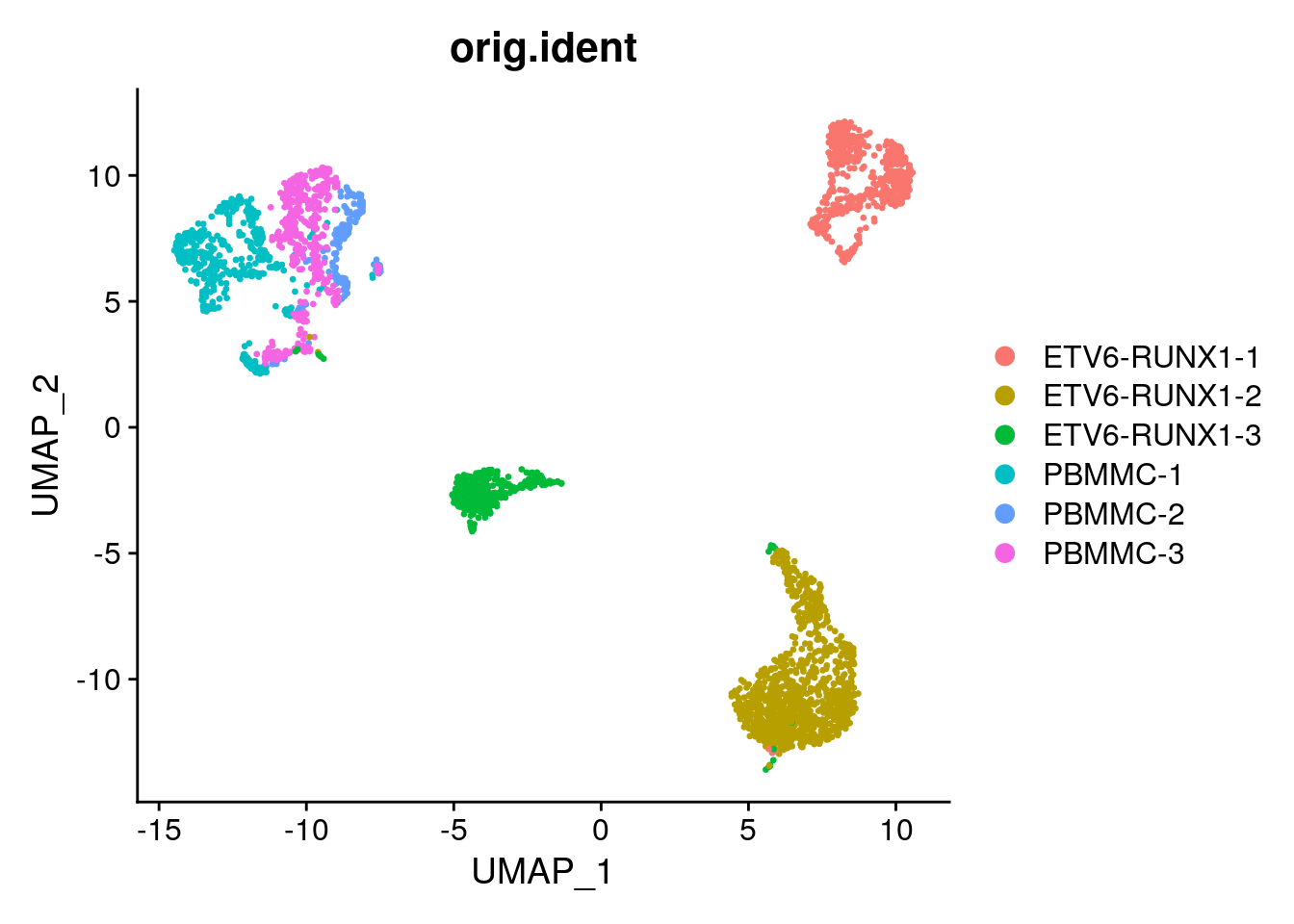
We can load the object and explore its UMAP and meta.data like this:
table(proB@meta.data$type)
ETV6-RUNX1 PBMMC
2000 1021 head(proB@meta.data) orig.ident nCount_RNA nFeature_RNA SingleR_annot
PBMMC-1_AAATGCCAGACTGGGT-1 PBMMC-1 4886 1727 Pro-B_cell_CD34+
PBMMC-1_AAATGCCTCCACTGGG-1 PBMMC-1 8397 2291 Pro-B_cell_CD34+
PBMMC-1_AACACGTTCTTGACGA-1 PBMMC-1 3444 1204 Pro-B_cell_CD34+
PBMMC-1_AACCATGAGAAGGTGA-1 PBMMC-1 8981 2437 Pro-B_cell_CD34+
PBMMC-1_AACCGCGCATGGTCAT-1 PBMMC-1 3719 1368 Pro-B_cell_CD34+
PBMMC-1_AAGCCGCCAGACGTAG-1 PBMMC-1 4573 1464 Pro-B_cell_CD34+
type
PBMMC-1_AAATGCCAGACTGGGT-1 PBMMC
PBMMC-1_AAATGCCTCCACTGGG-1 PBMMC
PBMMC-1_AACACGTTCTTGACGA-1 PBMMC
PBMMC-1_AACCATGAGAAGGTGA-1 PBMMC
PBMMC-1_AACCGCGCATGGTCAT-1 PBMMC
PBMMC-1_AAGCCGCCAGACGTAG-1 PBMMC
Note
If you want to know how this pro-B cell subset is generated, have a look at the script here.
Let’s have a look at the UMAP (again), coloured by celltype:
Seurat::DimPlot(proB, group.by = "type")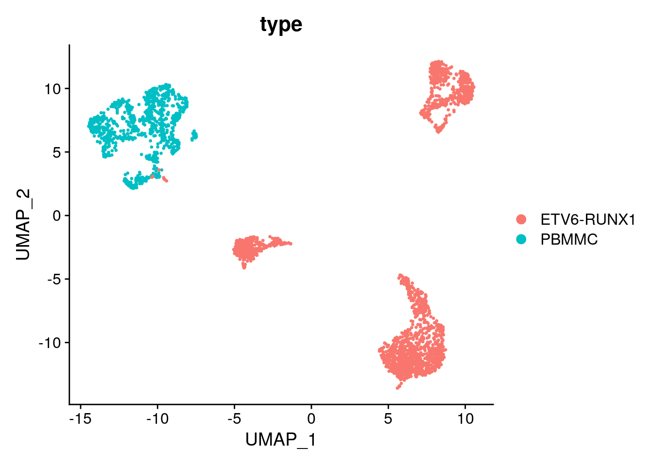
Let’s say we are specifically interested to test for differential gene expression between the tumor and normal samples.
Note
Here we could also test for e.g. healthy versus diseased within a celltype/cluster.
Now we will run differential expression analysis between tumor and healthy cells using the patient ID as a covariate by using limma.
Prepare the pseudobulk count matrix:
#taking the proB data
Seurat::DefaultAssay(proB) <- "RNA"
Seurat::Idents(proB) <- proB$orig.ident
## add the patient id also for paired DGE
proB$patient.id<-gsub("ETV6-RUNX1", "ETV6_RUNX1", proB$orig.ident)
proB$patient.id<-sapply(strsplit(proB$patient.id, "-"), '[', 2)
## Here we do perform pseudo-bulk:
##first a mandatory column of sample needs to be added to the meta data that is the grouping factor, should be the samples
proB$sample <- factor(proB$orig.ident)
# aggergate the cells per sampple
bulk <- Seurat::AggregateExpression(proB, group.by = "sample",
return.seurat = TRUE,
assay = "RNA")
# create a metadata data frame based on the aggregated cells
meta_data <- unique(proB@meta.data[, c("orig.ident",
"sample", "type",
"patient.id")])
rownames(meta_data) <- meta_data$orig.ident
bulk@meta.data <- meta_data[colnames(bulk), ]##have a look at the counts
counts <- Seurat::GetAssayData(bulk, layer = "counts") |> as.matrix()
head(counts) ETV6-RUNX1-1 ETV6-RUNX1-2 ETV6-RUNX1-3 PBMMC-1 PBMMC-2 PBMMC-3
RP11-34P13.7 0 0 0 2 0 0
FO538757.3 0 0 0 0 0 0
FO538757.2 138 275 74 129 40 112
AP006222.2 63 43 17 38 19 26
RP4-669L17.10 5 10 3 0 1 1
RP5-857K21.4 0 0 0 0 0 2#have a look at the colData of our new object summed, can you see type and
#patient.id are there
head(bulk@meta.data) orig.ident sample type patient.id
ETV6-RUNX1-1 ETV6-RUNX1-1 ETV6-RUNX1-1 ETV6-RUNX1 1
ETV6-RUNX1-2 ETV6-RUNX1-2 ETV6-RUNX1-2 ETV6-RUNX1 2
ETV6-RUNX1-3 ETV6-RUNX1-3 ETV6-RUNX1-3 ETV6-RUNX1 3
PBMMC-1 PBMMC-1 PBMMC-1 PBMMC 1
PBMMC-2 PBMMC-2 PBMMC-2 PBMMC 2
PBMMC-3 PBMMC-3 PBMMC-3 PBMMC 3Generate a DGEList object to use as input for limma and filter the genes to remove lowly expressed genes. How many are left?
#As in the standard limma analysis generate a DGE object
y <- edgeR::DGEList(counts, samples = bulk@meta.data)
##filter lowly expressed (recommanded for limma)
keep <- edgeR::filterByExpr(y, group = bulk$type)
y <- y[keep,]
##see how many genes were kept
summary(keep) Mode FALSE TRUE
logical 11086 10017 Generate a design matrix, including patient ID to model for a paired analysis. If you need help to generate a design matrix, check out the very nice edgeR User Guide, sections 3.3 and 3.4. Extract the sample ID from the meta.data, then create the design matrix:
## Create the design matrix and include the technology as a covariate:
design <- model.matrix(~0 + y$samples$type + y$samples$patient.id)
# Have a look
design y$samples$typeETV6-RUNX1 y$samples$typePBMMC y$samples$patient.id2
1 1 0 0
2 1 0 1
3 1 0 0
4 0 1 0
5 0 1 1
6 0 1 0
y$samples$patient.id3
1 0
2 0
3 1
4 0
5 0
6 1
attr(,"assign")
[1] 1 1 2 2
attr(,"contrasts")
attr(,"contrasts")$`y$samples$type`
[1] "contr.treatment"
attr(,"contrasts")$`y$samples$patient.id`
[1] "contr.treatment"# change column/rownames names to more simple group names:
colnames(design) <- make.names(c("ETV6-RUNX1", "PBMMC","patient2","patient3"))
rownames(design) <- rownames(y$samples)Specify which contrast to analyse:
contrast.mat <- limma::makeContrasts(ETV6.RUNX1 - PBMMC,
levels = design)Firt, we perform TMM normalization using edgeR, and then limma can perform the transformation with voom, fit the model, compute the contrasts and compute test statistics with eBayes:
dge <- edgeR::calcNormFactors(y)
#Do limma
vm <- limma::voom(dge, design = design, plot = TRUE)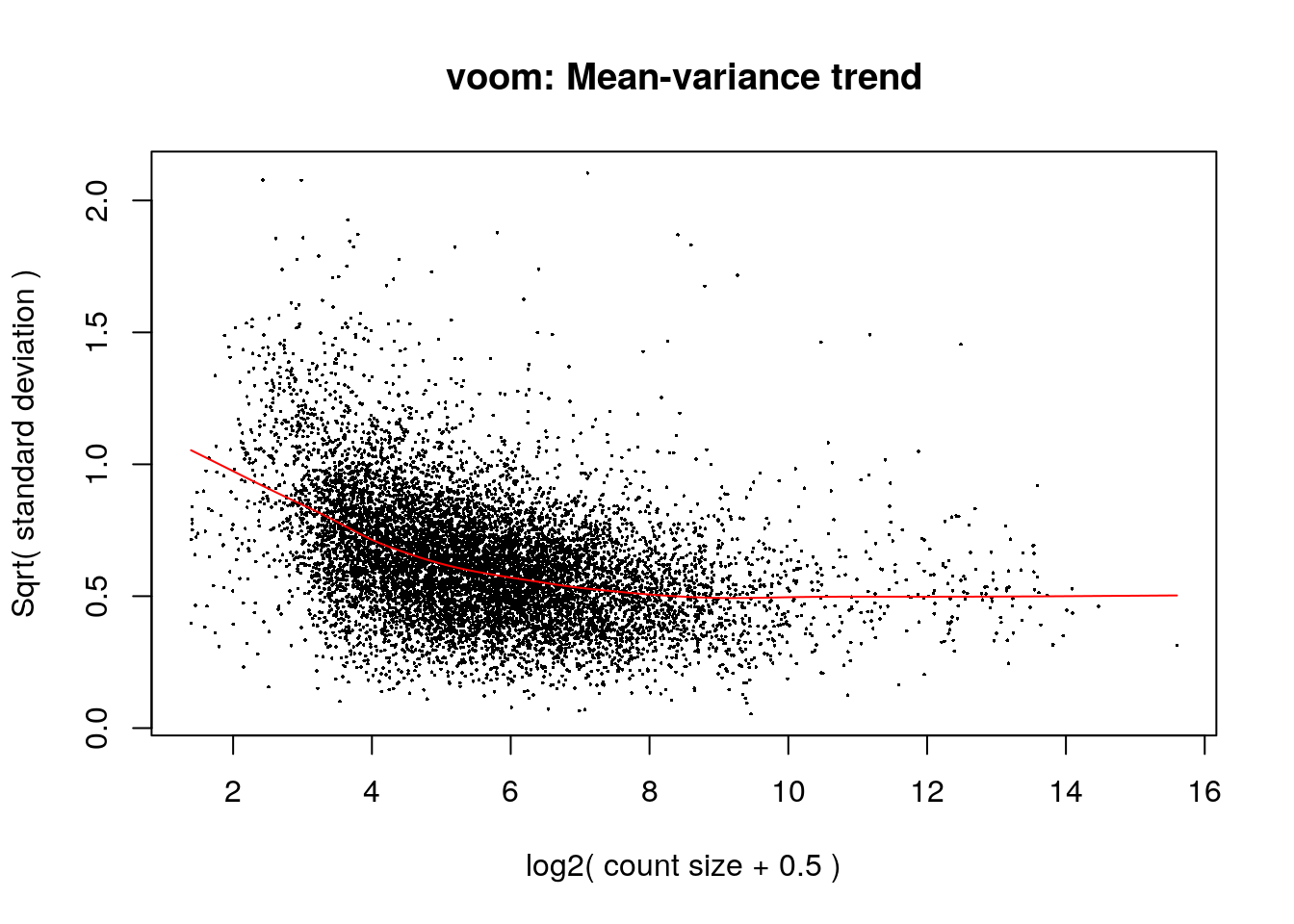
fit <- limma::lmFit(vm, design = design)
fit.contrasts <- limma::contrasts.fit(fit, contrast.mat)
fit.contrasts <- limma::eBayes(fit.contrasts)We can use topTable to get the most significantly differentially expressed genes, and save the full DE results to an object. How many genes are significant? Are you suprised by this number?
# Show the top differentially expressed genes:
limma::topTable(fit.contrasts, number = 10, sort.by = "P") logFC AveExpr t P.Value adj.P.Val B
RPS4Y2 5.346800 6.347826 15.39674 3.361453e-08 0.0001152727 9.477129
SDC2 9.070465 2.708711 15.33434 3.493119e-08 0.0001152727 7.681010
IGLL1 -3.788160 9.287148 -15.19483 3.808426e-08 0.0001152727 9.465422
CTGF 4.368363 6.029640 14.89301 4.603081e-08 0.0001152727 9.141505
AP005530.2 8.770808 2.560369 14.27130 6.879238e-08 0.0001335825 7.294079
GNG11 3.500250 6.457777 13.70183 1.008304e-07 0.0001335825 8.495288
HLA-DQA1 2.982748 7.410939 13.39202 1.249067e-07 0.0001335825 8.287394
PTP4A3 3.734865 5.449894 13.23439 1.395246e-07 0.0001335825 8.126807
CD27 4.115561 5.843582 13.23011 1.399471e-07 0.0001335825 8.147433
ALOX5 4.142010 5.682900 13.16658 1.463814e-07 0.0001335825 8.098199limma_de <- limma::topTable(fit.contrasts, number = Inf, sort.by = "P")
length(which(limma_de$adj.P.Val<0.05))[1] 2738And we can check whether this corresponds to the counts by generating a violin plot, or a gene downregulated in tumor, or a gene upregulated in tumor:
Seurat::VlnPlot(proB, "S100A9", split.by = "type")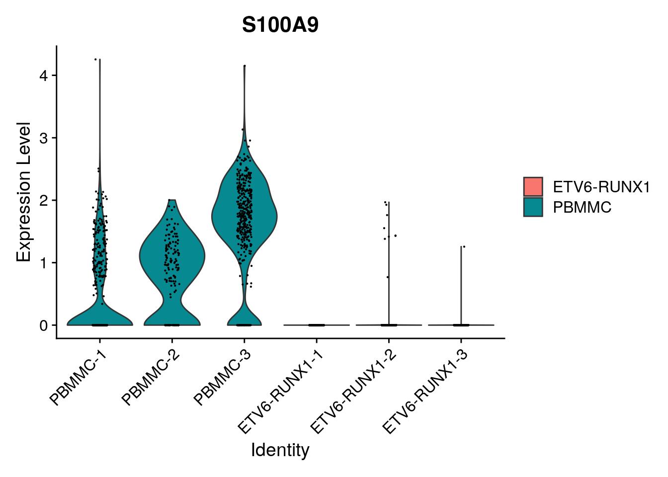
Seurat::VlnPlot(proB, "SOCS2", split.by = "type")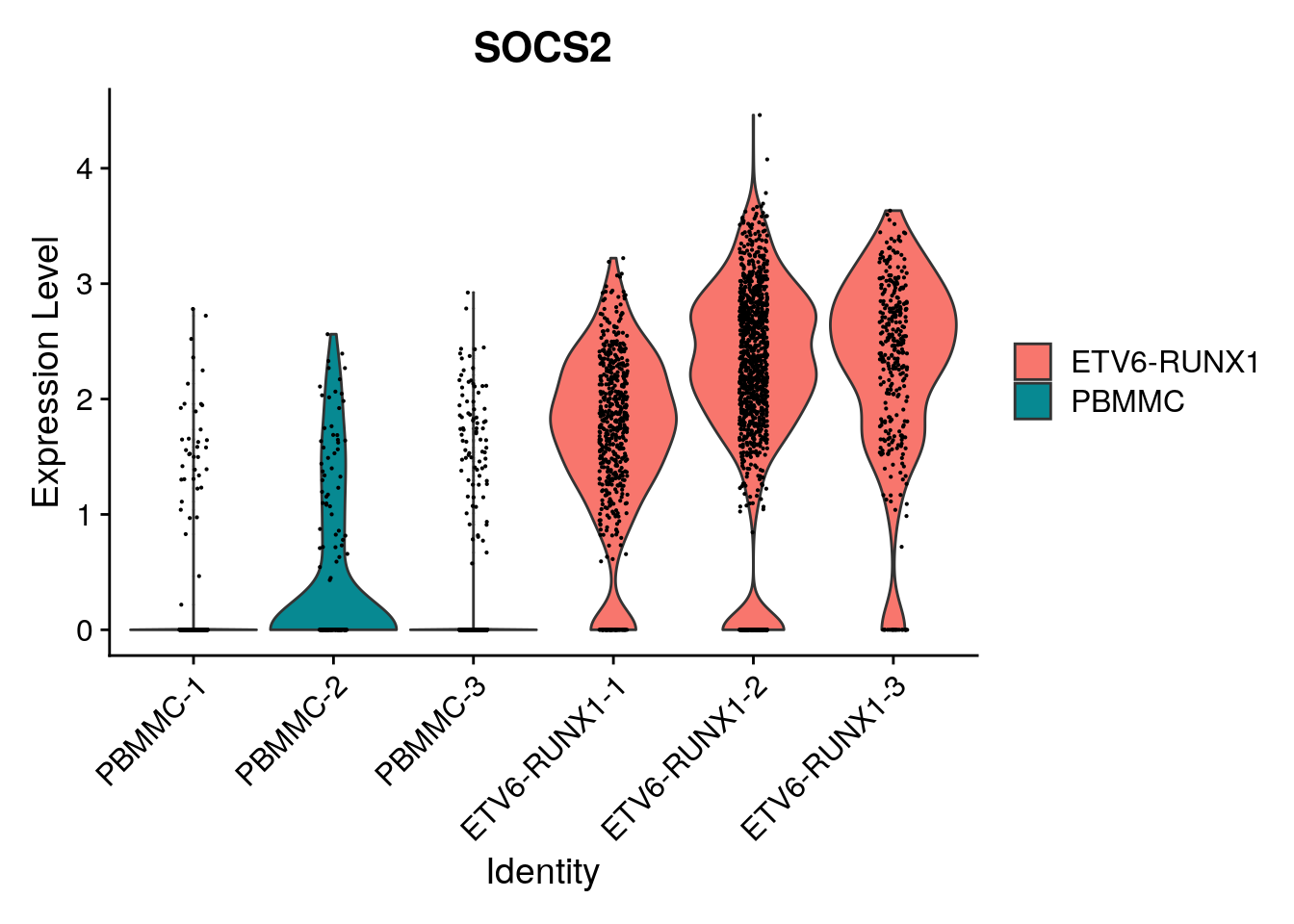
We can run a similar analysis with Seurat, but this will not take into account the paired design. Run the code below.
tum_vs_norm <- Seurat::FindMarkers(proB,
ident.1 = "ETV6-RUNX1",
ident.2 = "PBMMC",
group.by = "type")
tum_vs_norm <- subset(tum_vs_norm, tum_vs_norm$p_val_adj<0.05)
Exercise (extra)
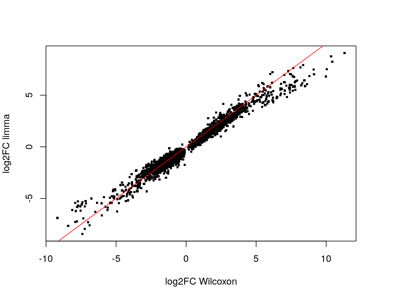
How many genes are significant? How does the fold change of these genes compare to the fold change of the top genes found by limma?
Answer
dim(tum_vs_norm) [1] 3820 5We find 3820 significant genes. If we merge the FindMarkers and the limma results, keep limma’s most significant genes and plot:
Keep the object
Keep the tum_vs_norm and limma_de objects because we will use this output later for the enrichment analysis in the next section.