Integration

Material

Exercises

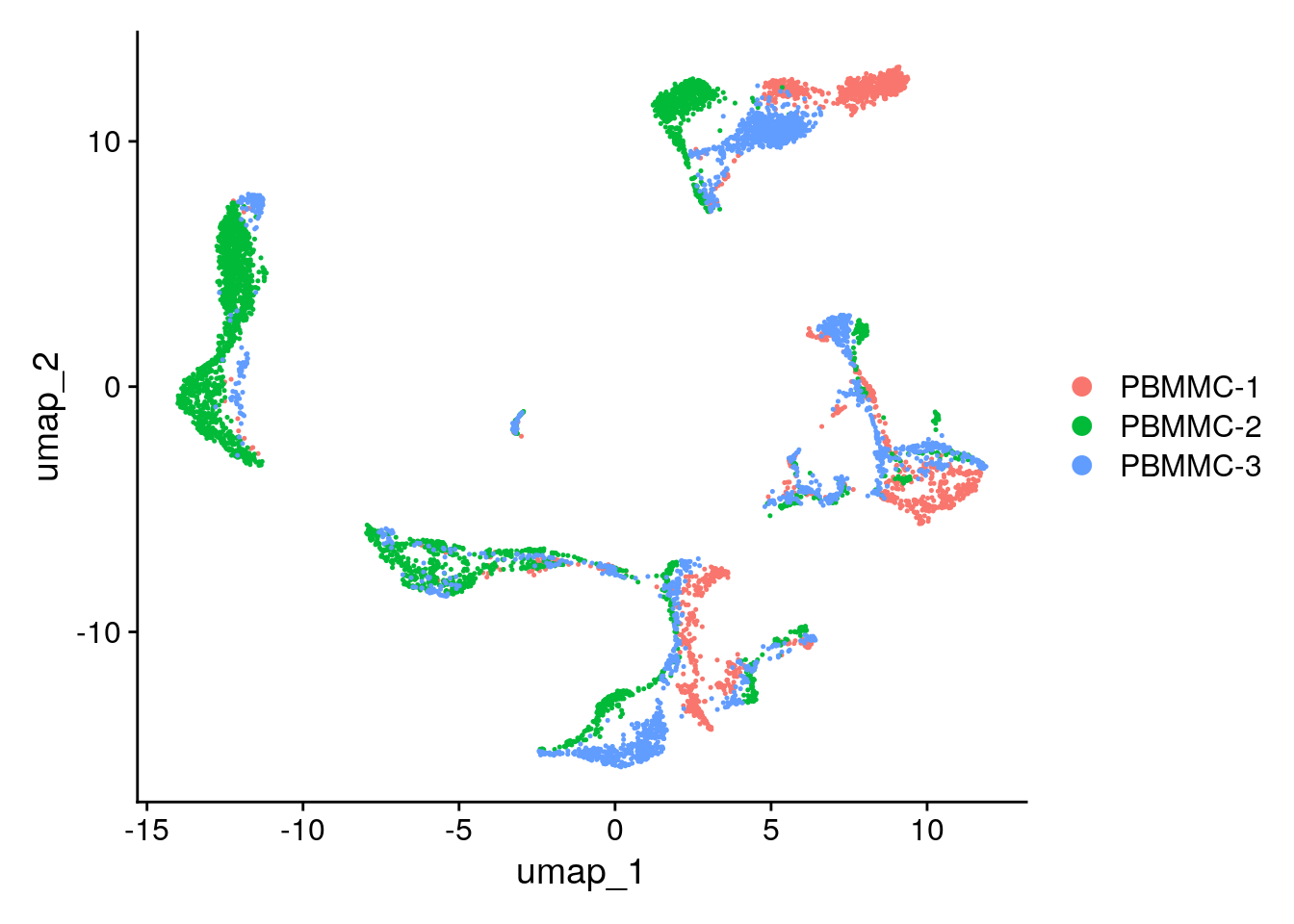
Let’s have a look at the UMAP again. Although cells of different samples are shared amongst ‘clusters’, you can still see seperation within the clusters:

Seurat::DimPlot(seu, reduction = "umap")

To perform the integration, we split our object by sample, resulting into a set of layers within the RNA assay. The layers are integrated and stored in the reduction slot - in our case we call it integrated.cca. Then, we re-join the layers

seu[["RNA"]] <- split(seu[["RNA"]], f = seu$orig.ident)

seu <- Seurat::IntegrateLayers(object = seu, method = CCAIntegration,
                       orig.reduction = "pca",
                       new.reduction = "integrated.cca",
                       verbose = FALSE)

# re-join layers after integration
seu[["RNA"]] <- JoinLayers(seu[["RNA"]])

We can then use this new integrated matrix for clustering and visualization. Now, we can re-run and visualize the results with UMAP.

Exercise

Create the UMAP again on the integrated.cca reduction (using the function RunUMAP - set the option reduction accordingly). After that, generate the UMAP plot. Did the integration perform well?

Answer

Performing the scaling, PCA and UMAP:

seu <- RunUMAP(seu, dims = 1:30, reduction = "integrated.cca")

Plotting the UMAP:

Seurat::DimPlot(seu, reduction = "umap")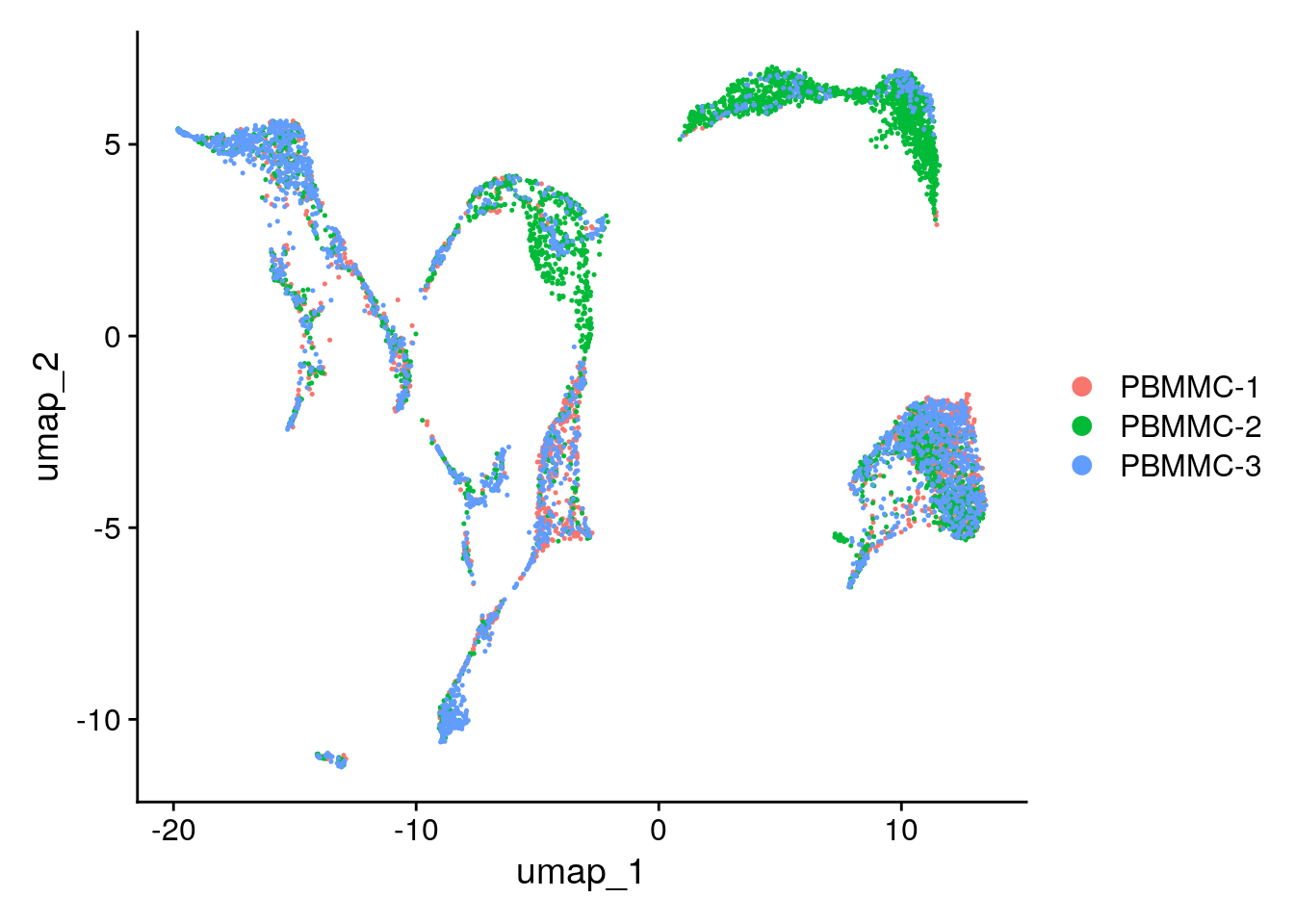

Save the dataset and clear environment

saveRDS(seu, "seu_day2-2.rds")

Clear your environment:

rm(list = ls())
gc()
.rs.restartR()