# Don't run it yet! Read the exercise first
seu <- Seurat::NormalizeData(seu,
                     normalization.method = "LogNormalize",
scale.factor = 10000)Normalization and scaling
Learning outcomes
After having completed this chapter you will be able to:
- Describe and perform standard procedures for normalization and scaling with the package
Seurat - Select the most variable genes from a
Seuratobject for downstream analyses
Material
Exercises
Normalization
After removing unwanted cells from the dataset, the next step is to normalize the data. By default, Seurat employs a global-scaling normalization method "LogNormalize" that normalizes the feature expression measurements for each cell by the total expression, multiplies this by a scale factor (10,000 by default), and log-transforms the result. Normalized values are stored in the “RNA” assay (as item of the @assay slot) of the seu object.
This is how you can call the function (don’t run it yet! Read the exercise first):
Exercise
Have a look at the assay data before and after running NormalizeData(). Did it change?
Tip
You can extract assay data with the function Seurat::GetAssayData. By default, the slot data is used (inside the slot assay), containing normalized counts. Use Seurat::GetAssayData(seu, slot = "counts") to get the raw counts.
Answer
You can check out some assay data with:
Seurat::GetAssayData(seu)[1:10,1:10] Returning:
Warning in GetAssayData.StdAssay(object = object[[assay]], layer = layer): data
layer is not found and counts layer is used
10 x 10 sparse Matrix of class "dgCMatrix" [[ suppressing 10 column names 'PBMMC-1_AAACCTGCAGACGCAA-1', 'PBMMC-1_AAACCTGTCATCACCC-1', 'PBMMC-1_AAAGATGCATAAAGGT-1' ... ]]
RP11-34P13.7  . . . . . . . . . .
FO538757.3    . . . . . . . . . .
FO538757.2    1 . . . . . 2 . . .
AP006222.2    . . . . . . . . . .
RP4-669L17.10 . . . . . . . . . .
RP5-857K21.4  . . . . . . . . . .
RP11-206L10.9 . . . . . . . . . .
LINC00115     . . . . . . . . . .
FAM41C        . . . . . . . . . .
RP11-54O7.1   . . . . . . . . . .
Normalizing layer: counts10 x 10 sparse Matrix of class "dgCMatrix" [[ suppressing 10 column names 'PBMMC-1_AAACCTGCAGACGCAA-1', 'PBMMC-1_AAACCTGTCATCACCC-1', 'PBMMC-1_AAAGATGCATAAAGGT-1' ... ]]
RP11-34P13.7  .        . . . . . .        . . .
FO538757.3    .        . . . . . .        . . .
FO538757.2    1.641892 . . . . . 1.381104 . . .
AP006222.2    .        . . . . . .        . . .
RP4-669L17.10 .        . . . . . .        . . .
RP5-857K21.4  .        . . . . . .        . . .
RP11-206L10.9 .        . . . . . .        . . .
LINC00115     .        . . . . . .        . . .
FAM41C        .        . . . . . .        . . .
RP11-54O7.1   .        . . . . . .        . . .
Updating
seu
As you might have noticed, this function takes the object seu as input, and it returns it to an object named seu. We can do this because the output of such calculations are added to the object, without loosing information.
Variable features
We next calculate a subset of features that exhibit high cell-to-cell variation in the dataset (i.e, they are highly expressed in some cells, and lowly expressed in others). Focusing on these genes in downstream analysis helps to highlight biological signal in single-cell datasets. The procedure in Seurat models the mean-variance relationship inherent in single-cell data, and is implemented in the FindVariableFeatures() function. By default, 2,000 genes (features) per dataset are returned and these will be used in downstream analysis, like PCA.
seu <- Seurat::FindVariableFeatures(seu,
                            selection.method = "vst",
                            nfeatures = 2000)
Finding variable features for layer countsLet’s have a look at the 10 most variable genes:
# Identify the 10 most highly variable genes
top10 <- head(Seurat::VariableFeatures(seu), 10)
top10
[1] "IGKC" "HBG2" "IGHG3" "IGHG1" "JCHAIN" "HBG1" "IGHA1" "IGHGP"
[9] "IGLC2" "IGLC3" We can plot them in a nicely labeled scatterplot:
vf_plot <- Seurat::VariableFeaturePlot(seu)
Seurat::LabelPoints(plot = vf_plot,
            points = top10, repel = TRUE)
When using repel, set xnudge and ynudge to 0 for optimal results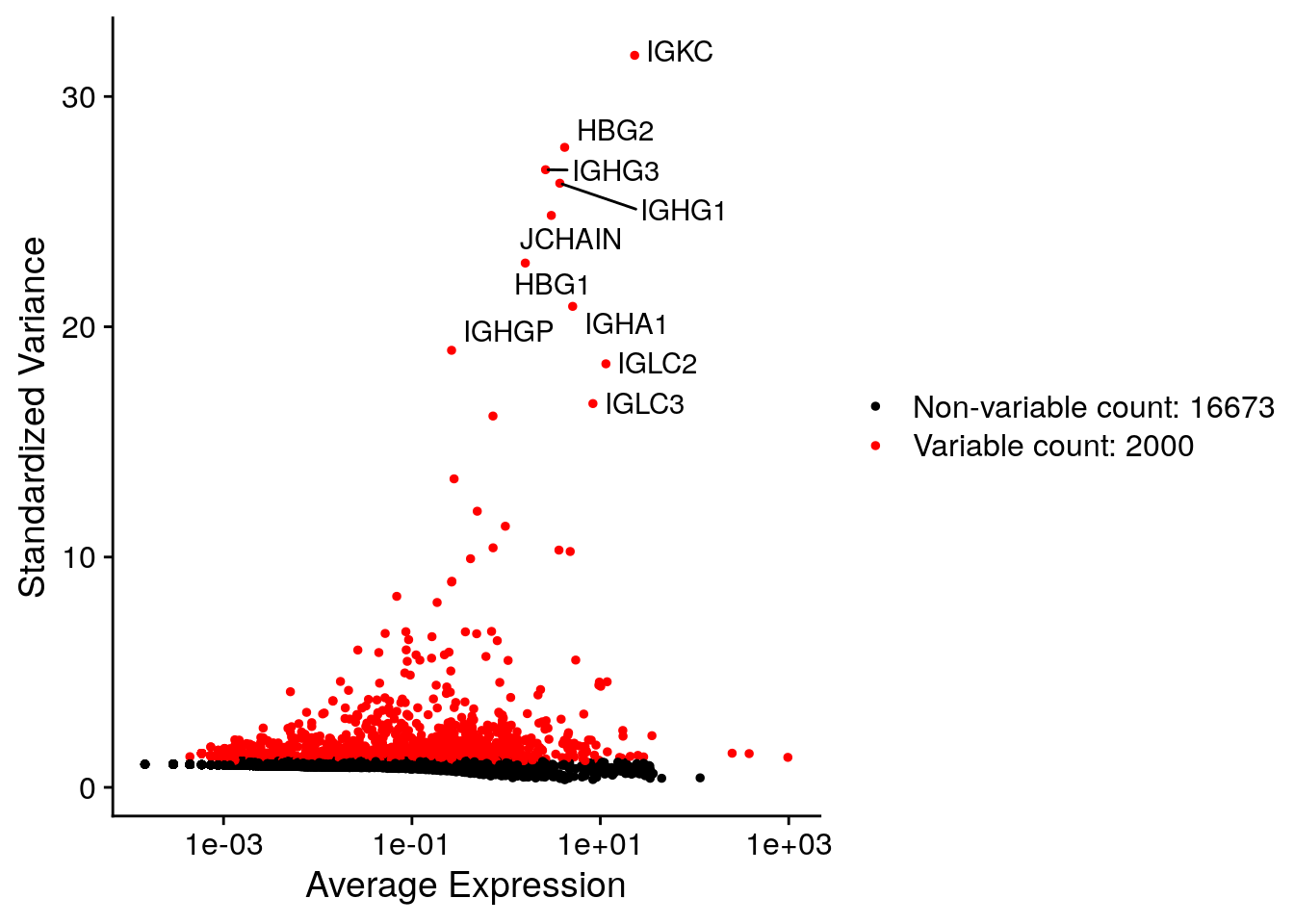
Make sure the plotting window is large enough
The function LabelPoints will throw an error if the plotting window is to small. If you get an error, increase plotting window size in RStudio and try again.
You can see that most of the highly variables are antibody subunits (starting with IGH, IGL). Not very surprising since we look at bone marrow tissue. We can have a look later in which cells they are expressed.
Scaling
Next, we apply scaling, a linear transformation that is a standard pre-processing step prior to dimensional reduction techniques like PCA. The ScaleData() function
- shifts the expression of each gene, so that the mean expression across cells is 0
- scales the expression of each gene, so that the variance across cells is 1
This step gives equal weight in downstream analyses, so that highly-expressed genes do not dominate. The results of this are stored in seu$RNA@scale.data
seu <- Seurat::ScaleData(seu)Centering and scaling data matrix
The use of
Seurat::SCTransform
The functions NormalizeData, VariableFeatures and ScaleData can be replaced by the function SCTransform. The latter uses a more sophisticated way to perform the normalization and scaling, and is argued to perform better. However, it is slower, and a bit less transparent compared to using the three separate functions. Therefore, we chose not to use SCTransform for the exercises.
Bonus exercise
Run SCTransform on the seu object. Where is the output stored?
Answer
You can run it like so:
seu <- Seurat::SCTransform(seu)And it will add an extra assay to the object. names(seu@assays) returns:
[1] "RNA" "SCT"Meaning that a whole new assay was added (including the sparse matrices with counts, normalized data and scaled data).
Warning
Running SCTransform will change @active.assay into SCT(in stead of RNA; check it with DefaultAssay(seu)). This assay is used as a default for following function calls. To change the active assay to RNA run:
DefaultAssay(seu) <- "RNA"Save the dataset and clear environment
Now, save the dataset so you can use it tomorrow:
saveRDS(seu, "seu_day1-3.rds")Clear your environment: